Physicspupil – Page 37

April 24, 2020February 5, 2023

202004240713 Homework 1 (Q3)

Suppose $G$ be a finite group of even order. Prove that there exists an element $a\in G$ such that $a\neq e$ and $a^2=e$ .

Attempts.

Try negating the statement by the following:

$\forall\, a\in G$ , either $a=e$ or $a^2\neq e$ ,

then looking for contradiction to the assumption that $G$ should be a finite group of even order.

CASE 1: Would it be possible that $a=e$ ?

Given so, the inverse and the identity of $G$ would be $e$ . And the set $G$ would have contained $e$ only, i.e., the singleton set $G=\{ e\}$ . This contradicts with the assumption that its order be even.

CASE 2: If for all elements in the group $G$ , their order cannot ever be $2$ .

If $a^2\neq e$ , then $a\neq a^{-1}$ for all $a\in G$ . It would then become an ill-posited negation, because the identity element $e$ is one of all $a\in G$ , and both statements $e^2\neq e$ and $e\neq e^{-1}$ are abhorrent to the basic axioms of a group. So perhaps to my discretion $e$ should be precluded from $a$ ‘s, and understood as one ( $e=e^{-1}$ ) member apart from the other members.

Proceeding to observe that if $a\neq a^{-1}$ for all $a\in G$ , I may then construct a pair of $a_i$ and $a_i^{-1}$ for $i\in \{ 1,2,\dots ,n:n\in\mathbb{Z}^+\}$ , provided from the definition of a group that the inverse of each element must exist and, as it follows, that it must be unique. That is, if $a_5=a_{27}^{-1}$ , I may relabel $a_{27}$ as $a_5^{-1}$ . By such a construction I can guarantee that all elements, except the identity $e$ , are now in pairs.

One therefore, by counting in total how many elements there are in group $G$ , will get an odd number $(2n+1)$ , the $2n$ counted from the pairs, and the single $1$ the identity $e$ itself alone counts.

This contradicts with the assumption that $|G|$ be of even parity.

From the negation of statement arises contradiction, the original statement is therefore proven by contradiction.

Remark.

I could not prove otherwise than loosely to so naive myself. Not until I had survived mathematical rigor.

April 24, 2020October 24, 2022

202004240630 Homework 1 (Q2)

Call $G$ a group and $e$ the identity of $G$ . If the order of $G$ is $2$ , then $a^2=e$ for all $a\in G$ and $G$ is abelian (Prove it yourself). Show that

$G$ is abelian if $a^2=e$ for all $a\in G$ .

Give an example of such a group whose order is greater than $2$ .

Solution.

Recall that a group $G$ is said to be abelian if $xy=yx$ for all $x,y\in G$ .

For any $a,b\in G$ , there is $ab=(bb^{-1})ab(a^{-1}a)$ , because a group satisfies, first, the inverse axiom $xx^{-1}=x^{-1}x=e$ under the notation $x^{-1}$ being the inverse of $x$ , and secondly, the identity axiom $ex=xe=x$ .

Thence by (associativity axiom) $x*(y*z)=(x*y)*z$ I may change brackets and obtain as follows:

$\begin{aligned} ab & =(bb^{-1})ab(a^{-1}a) \\ & =b(b^{-1}a)(ba^{-1})a \\ & =b(b^{-1}a)(b^{-1}a)^{-1}a \end{aligned}$

Provided that $a^2=e$ for all $a\in G$ , one may deduce $a=a^{-1}$ , $b=b^{-1}$ , etc. Thus,

$ab=b(b^{-1}a)(b^{-1}a)a$

In addition $(b^{-1}a)(b^{-1}a)=(b^{-1}a)^2=e$ , hence $ab=ba$ , and $G$ abelian.

The product group $\mathbb{Z}_2\times \mathbb{Z}_2$ is an example of one abelian group whose order is greater than $2$ and the order of whose elements is $2$ .

April 24, 2020October 24, 2022

202004240606 Homework 1 (Q1)

Let $G=\{ a,b,c,d\}$ and the Cayley table of $G$ be

$\begin{aligned} * \quad | &\textrm{} \quad a &\textrm{}\quad b \quad &\textrm{}\quad c &\textrm{}\quad d \\ \hline a \quad | &\quad a &\quad b \quad &\quad c &\quad d \\ b \quad | &\quad b &\quad a \quad &\quad c &\quad d \\ c \quad | &\quad c &\quad b \quad &\quad a &\quad d \\ d \quad | &\quad d &\quad d \quad &\quad b &\quad c \end{aligned}$

Is $(G,*)$ a group?

Attempts.

I recall that a group $(G,*)$ is a set $G$ altogether with an operation $*:G\times G\rightarrow G$ , $(x,y)\mapsto x*y$ such that the following axioms be satisfied:

i. (Associativity) $(x*y)*z=x*(y*z)$ ;

ii. (Identity) There exists $e\in G$ such that $e*x=x*e=x$ for all $x\in G$ ; and

iii. (Inverse) For each $a\in G$ , there exists $b\in G$ such that $a*b=b*a=e$ .

Let me check them one by one.

i. For $x,y,z\in \{ a,b,c,d \}$ , it suffices to check $4\times 4\times 4=64$ operations. And I found that the following operation failed axiom (i):

$d*(c*b)=d*b=d$ but $(d*c)*b=b*b=a$ .

That said, $G$ under the operation $*$ is not a group.

ii. By inspection, the identity of $G$ exists, and that is $a$ because $a*x=x*a=x$ for all $x\in \{ a,b,c,d\}$ . Axiom (ii) is thus satisfied.

iii. There exists $d\in G$ , such that for all $x^i\in\{ a,b,c,d\}=G$ ,

$d*x^i=x^i*d\neq a$ .

The claim above is validated by simply checking the identity found to be $a$ in part ii. cannot be found in the entries, and by the fact that $a$ is unique.

Axioms i. and iii. having been failed, I may conclude that $G$ under the operation $*$ cannot form a group.

April 24, 2020October 24, 2022

202004240535 Homework 1 (Q4)

What is the effective temperature of a neutron star with radius $10^6\,\mathrm{cm}$ which is detected to emit an energy flux $F=9\times 10^{-15}\,\mathrm{erg\, s^{-1}\, cm^{-2}}$ ? The distance to this neutron star is $1\,\mathrm{kpc}$ .

Setup.

Recall that the effective temperature $T_{\textrm{eff}}$ of a blackbody defines the frequency-integrated intensity of radiation at the source:

$\sigma_{\textrm{SB}}T^4_{\textrm{eff}}=F=\displaystyle{\int}I_\nu\cos\theta\,\mathrm{d}\nu\,\mathrm{d}\Omega$

where $\sigma_{\textrm{SB}}=5.67\times 10^{-5}\,\mathrm{erg\cdot cm^{-2}\, K^{-4}}$ is the Stefan-Boltzmann constant.

Solution. (guesstimate)

The luminosity $L$ of a source is related to the energy flux $F$ detected at some distance $d$ away from the source by

$F=\displaystyle{\frac{L}{4\pi d^2}}$ ,

from which one can infer the luminosity of the neutron star in question is

$\begin{aligned} L & =9\times 10^{-15}\times 4\pi (3.085677581\times 10^{21})^2 \\ & = 1.076845664\times 10^{30}\enspace \mathrm{erg\, s^{-1}} \end{aligned}$

where $d=1\,\mathrm{kpc}=3.085677581\times 10^{21}\,\mathrm{cm}$ is given.

Since $L=4\pi R^2\sigma_{\textrm{SB}}T_{\textrm{eff}}^4$ ,

$\begin{aligned} T^4_{\textrm{eff}} & =L/4\pi R^2\sigma_{\textrm{SB}} \\ T_{\textrm{eff}} & = \bigg(\frac{L}{4\pi R^2\sigma_{\textrm{SB}}}\bigg)^{1/4} \\ & = \bigg(\frac{1.076845664\times 10^{30}}{4\pi \times (10^6)^2\times 5.67\times 10^{-5}}\bigg)^{1/4} \\ T_{\textrm{eff}} & = 197169.6816\enspace \mathrm{K} \end{aligned}$

April 24, 2020October 24, 2022

202004240521 Homework 1 (Q5)

Estimate the apparent magnitude of Mercury and Venus when the Earth-planet-Sun forms a right angle. (Assuming the planet reflects 50% of solar light.)

Setup.

Recall the apparent magnitude $m_b$ , the Sun’s luminosity being the reference, is given by the formula

$m_b=-0.23+5\log D-2.5\log (L/L_{\odot})$ ,

where $D$ is the distance (in parsec) from the source to the Earth, $L$ the luminosity of the source, and $L_\odot =3.8\times 10^{33}\,\mathrm{erg\, s^{-1}}$ the solar luminosity.

CASE I of Mercury

According to http://coolcosmos.ipac.caltech.edu/ask/25-How-far-is-Mercury-from-Earth-, the average distance between Mercury and Earth is 0.0000024954 pc. From Wikipedia on Mercury (planet), the mean radius of Mercury $R_{\textrm{Mercury}}$ is $2439.7\pm 1\,\mathrm{km}$ .

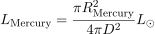
The luminosity of Mercury $L_{\textrm{Mercury}}$ due to reflection of sunlight, is related to the solar luminosity $L_\odot =3.8\times 10^{33}\,\mathrm{erg\, s^{-1}}$ by

$L_{\textrm{Mercury}}=\displaystyle{\frac{\pi R^2_{\textrm{Mercury}}}{4\pi D^2}}L_\odot$ ,

where the Sun-Earth distance $D$ is one astronomical unit $1\,\mathrm{AU}=1.5\times 10^{13}\,\mathrm{cm}$ .

Thence one computes

$\begin{aligned} L_{\textrm{Mercury}} & = \displaystyle{\frac{\pi (2.4397\times 10^8)^2}{4\pi (1.5\times 10^{13})^2}}\times 3.8\times 10^{33} \\ & = 2.513124127\times 10^{23}\enspace \mathrm{erg\, s^{-1}} \end{aligned}$

Thus, the apparent magnitude $m_{b,\textrm{mercury}}$ of Mercury is

$\begin{aligned} m_{b,\textrm{mercury}} & =-0.23+5\log (0.0000024954)-2.5\log (6.613484544\times 10^{-11})\\ & = -2.795375004 \end{aligned}$

CASE II of Venus

According to http://coolcosmos.ipac.caltech.edu/ask/52-How-far-away-is-Venus-from-Earth-, the average distance between Venus and Earth is 0.0000012963 pc. From Wikipedia on Venus, the mean radius of Venus $R_{\textrm{Venus}}$ is $6051.8\pm 1\,\mathrm{km}$ .

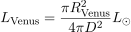
The luminosity of Venus $L_{\textrm{Venus}}$ due to reflection of sunlight, is related to the solar luminosity $L_\odot =3.8\times 10^{33}\,\mathrm{erg\, s^{-1}}$ by

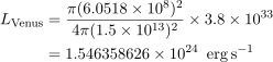
$L_{\textrm{Venus}}=\displaystyle{\frac{\pi R^2_{\textrm{Venus}}}{4\pi D^2}}L_\odot$ ,

where the Sun-Earth distance $D$ is one astronomical unit $1\,\mathrm{AU}=1.5\times 10^{13}\,\mathrm{cm}$ .

Thence one computes

$\begin{aligned} L_{\textrm{Venus}} & = \displaystyle{\frac{\pi (6.0518\times 10^8)^2}{4\pi (1.5\times 10^{13})^2}}\times 3.8\times 10^{33} \\ & = 1.546358626\times 10^{24}\enspace \mathrm{erg\, s^{-1}} \end{aligned}$

Thus, the apparent magnitude $m_{b,\textrm{venus}}$ of Venus is

$\begin{aligned} m_{b,\textrm{venus}} & =-0.23+5\log (0.0000012963)-2.5\log (4.069364804\times 10^{-10})\\ & = -6.190288956 \end{aligned}$

Correction.

Without heed to the 50% reduction of solar light reflection, this problem need be redone.

April 24, 2020October 24, 2022

202004240406 Homework 1 (Q6)

Derive the Planck function $B_\nu$ .

HINTS: You can make the following steps.

(1) Show that the density of states for photons is given by

$g(E)=\displaystyle{\frac{\mathrm{d}N}{\mathrm{d}E}=\frac{8\pi VE^2}{h^3c^3}}$ ,

(2) the photon density per unit frequency is given by

$\displaystyle{\frac{\mathrm{d}n}{\mathrm{d}\nu}}=\displaystyle{\frac{8\pi \nu^2}{c^3(e^{h\nu /kT+1})}}$ , and

(3) the definition of the specific intensity $B_\nu =I_\nu$ is the energy flux per unit frequency per unit solid angle.

Note: the energy and momentum of photons are related as

$E=h\nu =pc$ ,

the energy flux per unit frequency is given by

$h\nu \displaystyle{\frac{\mathrm{d}n}{\mathrm{d}\nu}}c$ ,

and total solid angle for isotropic emission is $4\pi$ .

Attempts.

In attempting to derive the Planck function, extensive reference was made to the following several sources found on the Internet:

i. G. B. Rybicki & A. P. Lightman. (1979). Radiative Processes in Astrophysics. John Wiley & Sons, Inc.

ii. https://edisciplinas.usp.br/pluginfile.php/48089/course/section/16461/qsp_chapter10-plank(DOT)pdf

iii. https://en.wikipedia(DOT)org/wiki/Planck\%27s_law#Derivation

iv. http://web.phys.ntnu.no/~stovneng/TFY4165_2013/BlackbodyRadiation(DOT)pdf

Here I follow Rybicki and Lightman’s derivation (pp. 20–22, 1979) direct, and have changed only some wordings.

Solution.

The wave vector of the photon of frequency $\nu$ propagating in direction $\mathbf{n}$ is $\mathbf{k}=(2\pi /\lambda )\,\mathbf{n}=(2\pi\nu /c)\,\mathbf{n}$ . For a photon gas in a box of dimension $(L_x,L_y,L_z)$ , the number of nodes of the standing wave is $n_i=k_iL_i/2\pi$ for each direction $i\in\{ x,y,z\}$ and for some wave number $k_i$ . For all directions, write the variation of the number of nodes with the wave number

$\Delta n_i=\displaystyle{\frac{L_i\Delta k_i}{2\pi}}$

The three-dimensional wave vector element $\Delta k_x\Delta k_y\Delta k_z\equiv \mathrm{d}^3k$ has the number of states to be

$\Delta N=\Delta n_x\Delta n_y\Delta n_z=\displaystyle{\frac{L_xL_yL_z\,\mathrm{d}^3k}{(2\pi )^3}}$

By the fact that $L_xL_yL_z=V$ is the volume of the box and the fact that photons have two independent polarizations (i.e., two states per wave vector $\mathbf{k}$ ), for each 3D-wave vector, the number of states for every unit volume is

$\displaystyle{\frac{\Delta N}{V\,\mathrm{d}^3k}}=2/(2\pi )^3$ .

Using solid angle as in spherical coordinates, rewrite

$\mathrm{d}^3k=k^2\,\mathrm{d}k\,\mathrm{d}\Omega =\displaystyle{\frac{(2\pi )^3\nu^2\,\mathrm{d}\nu\,\mathrm{d}\Omega}{c^3}}$ .

Then, the density of states, i.e., the number of states per solid angle per volume per frequency, is given by

$\rho_s\stackrel{\textrm{def}}{=}\displaystyle{\frac{\mathrm{d}N}{\mathrm{d}\Omega\,\mathrm{d}V\,\mathrm{d}\nu}}=\displaystyle{\frac{2\nu^2}{c^3}}$ .

As each state of $n$ photons each of energy $h\nu$ is of energy $E_n=nh\nu$ , and according to statistical mechanics the probability of a state of energy $E_n$ is proportional to $\mathrm{exp}(-\beta E_n)$ (where $\beta =1/kT$ and $k=\textrm{ the Boltzmann's constant}$ ), the average energy of each state is

$\overline{E}=\displaystyle{\frac{\sum_{n=0}^\infty E_n\mathrm{exp}(-\beta E_n)}{\sum_{n=0}^\infty \mathrm{exp}(-\beta E_n)}}=-\displaystyle{\frac{\mathrm{\partial}}{\mathrm{\partial}\beta}\ln \bigg( \sum_{n=0}^\infty \mathrm{exp}(-\beta E_n)\bigg)}$ .

Recall the formula for the sum of a geometric series:

$\displaystyle{\sum_{n=0}^\infty}\mathrm{exp}(-\beta E_n)=\displaystyle{\sum_{n=0}^\infty}\mathrm{exp}(-nh\nu\beta )=(1-\mathrm{exp}(-\beta h\nu ))^{-1}$ ,

one has therefore the result (in Bose-Einstein statistics)

$\overline{E}=\displaystyle{\frac{h\nu\,\mathrm{exp}(-\beta h\nu )}{1-\mathrm{exp}(-\beta h\nu )}=\frac{h\nu}{\mathrm{exp}(h\nu /kT)-1}}$ .

where it can be seen that the occupation number

$n_\nu =\bigg[ \mathrm{exp}\bigg( \displaystyle{\frac{h\nu}{kT}}\bigg) -1\bigg]^{-1}$

means the average number of photons in some frequency $\nu$ , as one energy $h\nu$ corresponds to one frequency $\nu$ .

The energy per solid angle per volume per frequency is the product of i. $\overline{E}$ , the average energy of each state, and ii. $\rho_s$ , the density of states.

I.e., $\overline{E}\cdot \rho_s = \bigg( \displaystyle{\frac{2\nu^2}{c^3}}\bigg) \displaystyle{\frac{h\nu}{\mathrm{exp}(h\nu /kT)-1}}$

Define the specific energy density $u_\nu$ the energy per unit volume per unit frequency range. Then the energy density per unit solid angle can be expressed as

$\begin{aligned} u_\nu (\Omega ) & =\displaystyle{\frac{\mathrm{d}E}{\mathrm{d}V\,\mathrm{d}\Omega\,\mathrm{d}\nu}} \\ \dots \textrm{arranging } & \textrm{and equating the previous two equations}\dots \\ u_\nu (\Omega )\,\mathrm{d}V\,\mathrm{d}\nu\,\mathrm{d}\Omega & =\bigg( \displaystyle{\frac{2\nu^2}{c^3}}\bigg) \displaystyle{\frac{h\nu}{\mathrm{exp}(h\nu /kT)-1}}\,\mathrm{d}V\,\mathrm{d}\nu\,\mathrm{d}\Omega \\ \dots \textrm{comparing} & \dots \\ u_\nu (\Omega ) & = \bigg( \displaystyle{\frac{2\nu^2}{c^3}}\bigg) \displaystyle{\frac{h\nu}{\mathrm{exp}(h\nu /kT)-1}} \end{aligned}$

Observe that the specific energy density $u_\nu$ and the specific intensity (or brightness) $I_\nu$ are related by

$u_\nu (\Omega )=\displaystyle{\frac{I_\nu}{c}}$ .

Now that the specific intensity, $I_\nu$ , is the same as the source function (of specific emission mechanism), $B_\nu$ .
The frequency distribution is said to be a blackbody form, i.e.,

The Planck function is expressed as

$\boxed{I_\nu =B_\nu (T)=\displaystyle{\frac{2h\nu^3}{c^2}}\bigg[ \mathrm{exp}\bigg( \displaystyle{\frac{h\nu}{kT}} \bigg) -1\bigg]^{-1}}$

(Units: $\mathrm{erg\cdot s^{-1}\cdot Hz^{-1}\cdot cm^{-2}\cdot ster^{-1}}$ )

April 23, 2020October 14, 2023

202004231606 Exercise 1, Section 1.1

Determine whether the vectors emanating from the origin and terminating at the following pair of points are parallel.

(a) $(3,1,2)$ and $(6,4,2)$

(b) $(-3,1,7)$ and $(9,-3,-21)$

(c) $(5,-6,7)$ and $(-5,6,-7)$

(d) $(2,0,-5)$ and $(5,0,-2)$

Background.

Two nonzero vectors $x$ and $y$ are called parallel if $y=tx$ for some nonzero real number $t$ . (Thus nonzero vectors having the same or opposite directions are parallel.)

_{Text on pg.3}

Solution.

(a) Let $x=(3,1,2)$ and $y=(6,4,2)$ . Apparently $\nexists\, t\in \mathbb{R}$ such that $y=tx$ . For otherwise $(6,4,2)=t(3,1,2)$ , the system of equations

$\begin{aligned} 6 & = 3t \\ 4 & = 1t \\ 2 & = 2t \\ \end{aligned}$

is inconsistent. They are not parallel.

(b) Let $x=(-3,1,7)$ and $y=(9,-3,-21)$ , then $y=-3x$ . The vectors $x$ and $y$ are in opposite direction and the magnitude of $y$ is three times that of $x$ . They are parallel.

(c) Let $x=(5,-6,7)$ and $y=(-5,6,-7)$ . Observe that they are in equal magnitude but in opposite direction, i.e., $y=-x$ . They are also parallel.

(d) Let $x=(2,0,-5)$ and $y=(5,0,-2)$ . Assume $t\in\mathbb{R}$ s.t. $y=tx$ , i.e.,

$\begin{aligned} 5 & = 2t \\ 0 & = 0t \\ -2 & = 5t \\ \end{aligned}$

no way will the first and the third lines agree. They are nonparallel.

November 19, 2019April 13, 2023

201911190435 Homework 1 (Q4)

A point particle moves in space under the influence of force derivable from a generalized potential of the form

$U(\mathbf{r},\mathbf{v})=V(r)+\sigma\cdot\textrm{\textbf{L}}$

where $\mathbf{r}$ is the radius vector from a fixed point, $\textrm{\textbf{L}}$ is the angular momentum about that point, and $\sigma$ is a fixed vector in space.

1. Find the components of the force on the particle in both Cartesian and spherical polar coordinates, on the basis of Eq. (1.58) in Goldstein’s book.

2. Show that the components in the two coordinates systems are related to each other as in Eq. (1.49) in Goldstein’s book.

3. Obtain the equation of motion in spherical polar coordinates.

Solution. (bad, probably wrong)

1.

i. In Cartesian coordinates $(x,y,z)$ , the potential $V(r)=V(x,y,z)$ . Here I take the definition of angular momentum $\mathbf{L}$ to be the vector product of position $\mathbf{r}=\mathbf{r}(x,y,z)$ and linear momentum $\mathbf{p}=(\mathbf{p}_x,\mathbf{p}_y,\mathbf{p}_z)$ : $\begin{aligned} \mathbf{L} & =\mathbf{r}\times \mathbf{p}=\begin{vmatrix} \hat{\mathbf{i}} & \hat{\mathbf{j}} & \hat{\mathbf{k}} \\ x & y & z \\ m\dot{x} & m\dot{y} & m\dot{z}\\ \end{vmatrix}\\ (L_x,L_y,L_z) & =m(y\dot{z}-z\dot{y},z\dot{x}-x\dot{z},x\dot{y}-y\dot{x})\end{aligned}$

In passing, is given as a fixed vector, thus it is, in particular, independent of position and vector , and, in general, independent of generalized coordinates and generalized velocities.

Goldstein’s Classical Mechanics, the generalized force is given by the equation below:

Eq. (1-54):

$Q_i=-\displaystyle{\frac{\partial U}{\partial q_i}}+\displaystyle{\frac{\mathrm{d}}{\mathrm{d}t}\bigg( \frac{\partial U}{\partial \dot{q_i}} \bigg)}$

In Cartesian coordinates, write the general potential in the form of
$U(x,y,z,\dot{x},\dot{y},\dot{z})=V(x,y,z)+\sigma\cdot (L_x,L_y,L_z)$ .
Compute the partial derivatives with respect to $x$ , $y$ , $z$ :
$\begin{aligned} \displaystyle{\frac{\partial U}{\partial x}} & = \partial_xV+\sigma\cdot \partial_x(L_x,L_y,L_z)\\ & = -F_x+\sigma\cdot m(0,-\dot{z},\dot{y}) \\ \displaystyle{\frac{\partial U}{\partial y}} & = \partial_yV+\sigma\cdot \partial_y(L_x,L_y,L_z)\\ & = -F_y+\sigma\cdot m(\dot{z},0,-\dot{x}) \\ \displaystyle{\frac{\partial U}{\partial z}} & = \partial_zV+\sigma\cdot \partial_z(L_x,L_y,L_z)\\ & = -F_z+\sigma\cdot m(-\dot{y},\dot{x},0)\\ \end{aligned}$
Compute the partial derivatives with respect to $\dot{x}$ , $\dot{y}$ , $\dot{z}$ :
$\begin{aligned} \displaystyle{\frac{\partial U}{\partial \dot{x}}} & = \sigma\cdot \partial_{\dot{x}}(L_x,L_y,L_z) \\ & = \sigma\cdot m(0,z,-y)\\ \displaystyle{\frac{\partial U}{\partial \dot{y}}} & = \sigma\cdot \partial_{\dot{y}}(L_x,L_y,L_z)\\ & = \sigma\cdot m(-z,0,x)\\ \displaystyle{\frac{\partial U}{\partial \dot{z}}} & = \sigma\cdot \partial_{\dot{z}}(L_x,L_y,L_z)\\ & = \sigma\cdot m(y,-x,0)\\ \end{aligned}$
Finally, taking total derivatives w.r.t. time $t$ on the preceding:
$\begin{aligned} \displaystyle{\frac{\mathrm{d}}{\mathrm{d}t}\bigg(\frac{\partial U}{\partial \dot{x}}\bigg)} & = \sigma\cdot m(0,\dot{z},-\dot{y})\\ \displaystyle{\frac{\mathrm{d}}{\mathrm{d}t}\bigg(\frac{\partial U}{\partial \dot{y}}\bigg)} & = \sigma\cdot m(-\dot{z},0,\dot{x})\\ \displaystyle{\frac{\mathrm{d}}{\mathrm{d}t}\bigg(\frac{\partial U}{\partial \dot{z}}\bigg)} & = \sigma\cdot m(\dot{y},-\dot{x},0)\\ \end{aligned}$
I shall obtain the following generalized forces:
$\begin{aligned} Q_x & = -\Big( -F_x+\sigma\cdot m(0,-\dot{z},\dot{y})\Big)+\Big(\sigma\cdot m(0,\dot{z},-\dot{y})\Big)\\ & = F_x+2\sigma m(0,\dot{z},-\dot{y})\\ Q_y & =-\Big( -F_y+\sigma\cdot m(\dot{z},0,-\dot{x})\Big)+\Big(\sigma\cdot m(-\dot{z},0,\dot{x})\Big)\\ & = F_y+2\sigma m(-\dot{z},0,\dot{x})\\ Q_z & =-\Big( -F_z+\sigma\cdot m(-\dot{y},\dot{x},0)\Big)+\Big(\sigma\cdot m(\dot{y},-\dot{x},0)\Big)\\ & = F_z+2\sigma m(\dot{y},-\dot{x},0)\\ \end{aligned}$
ii. In spherical (or, polar, as may be reduced) coordinates $(r,\theta ,\phi)$ we have the potential $V(r)$ with only $r$ -dependence. The angular momentum $\mathbf{L}$ is said to be $\mathbf{L}=m(\mathbf{r}\times\mathbf{v})$ , where the position $\mathbf{r}=\mathbf{r}(r,\theta ,\phi )$ and the velocity $\mathbf{v}=\mathbf{v}(r,\theta ,\phi)$ are in terms of spherical coordinates.
The transformation between spherical and Cartesian coordinates is:
$\begin{aligned} x & =r\sin\theta\cos\phi \\ y & =r\sin\theta\sin\phi \\ z & =r\cos\theta \\ \end{aligned}$ .
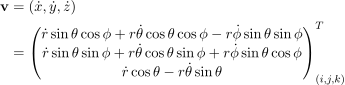
The velocity vector $\mathbf{v}$ may thus be represented as:
$\begin{aligned} \mathbf{v} & =(\dot{x},\dot{y},\dot{z})\\ & = \begin{pmatrix} \dot{r}\sin\theta\cos\phi +r\dot{\theta}\cos\theta\cos\phi -r\dot{\phi}\sin\theta\sin\phi \\ \dot{r}\sin\theta\sin\phi +r\dot{\theta}\cos\theta\sin\phi +r\dot{\phi}\sin\theta\cos\phi \\ \dot{r}\cos\theta -r\dot{\theta}\sin\theta \\ \end{pmatrix}^T_{(i,j,k)}\\ \end{aligned}$
Using the fact which was derived formerly:
$(L_x,L_y,L_z)=m(y\dot{z}-z\dot{y},z\dot{x}-x\dot{z},x\dot{y}-y\dot{x})$
and by some direct computation below
$\begin{aligned} & L_x/m \\ & = y\dot{z}-z\dot{y} \\ & = (r\sin\theta\sin\phi )(\dot{r}\cos\theta -r\dot{\theta}\sin\theta ) \\ &\qquad\qquad -(r\cos\theta )(\dot{r}\sin\theta\sin\phi +r\dot{\theta}\cos\theta\sin\phi +r\dot{\phi}\sin\theta\cos\phi )\\ & = -r^2\dot{\theta}\sin^2\theta\sin\phi -r^2\dot{\theta}\cos^2\theta\sin\phi +r^2\dot{\phi}\sin 2\theta\cos\phi \\ & = r^2(\dot{\phi}\sin 2\theta\cos\phi -\dot{\theta}\sin\phi )\\ \end{aligned}$
$\begin{aligned} & L_y/m\\ & = z\dot{x}-x\dot{z} \\ & = (r\cos\theta )(\dot{r}\sin\theta\cos\phi +r\dot{\theta}\cos\theta\cos\phi -r\dot{\phi}\sin\theta\sin\phi )\\ &\qquad\qquad -(r\sin\theta\cos\phi )(\dot{r}\cos\theta -r\dot{\theta}\sin\theta )\\ & = r^2\dot{\theta}\cos^2\theta \cos\phi -r^2\dot{\phi}\sin 2\theta\sin\phi +r^2\dot{\theta}\sin^2\theta\cos\phi \\ & = r^2(\dot{\theta}\cos\phi -\dot{\phi}\sin 2\theta\sin\phi )\\ \end{aligned}$
$\begin{aligned} & L_z/m \\ & = x\dot{y}-y\dot{x} \\ & = (r\sin\theta\cos\phi )(\dot{r}\sin\theta\sin\phi +r\dot{\theta}\cos\theta\sin\phi +r\dot{\phi}\sin\theta\cos\phi )\\ & \qquad -(r\sin\theta\sin\phi )(\dot{r}\sin\theta\cos\phi +r\dot{\theta}\cos\theta\cos\phi -r\dot{\phi}\sin\theta\sin\phi )\\ & =r^2\dot{\phi}\sin^2\theta\cos^2\phi +r^2\dot{\phi}\sin^2\theta\sin^2\phi \\ & = r^2\dot{\phi}\sin^2\theta \\ \end{aligned}$
then summing up what is up till now, the angular momentum $\mathbf{L}$ in terms of spherical coordinate components in Cartesian natural bases is
$\mathbf{L}=\begin{pmatrix} L_r \\ L_\theta \\ L_\phi \\ \end{pmatrix}^T=mr^2\begin{pmatrix} \dot{\phi}\sin 2\theta\cos\phi -\dot{\theta}\sin\phi \\ \dot{\theta}\cos\phi -\dot{\phi}\sin 2\theta\sin\phi \\ \dot{\phi}\sin^2\theta \\ \end{pmatrix}^T_{(i,j,k)}$
In spherical coordinates, write the general potential in the form of
$U(r,\theta ,\phi ,\dot{r},\dot{\theta},\dot{\phi})=V(r)+\sigma\cdot \mathbf{L}(L_r,L_\theta ,L_\phi )$ .
Then,
$\begin{aligned}[t] Q_r & =-\displaystyle{\frac{\partial U}{\partial r}}+\displaystyle{\frac{\mathrm{d}}{\mathrm{d}t}\bigg( \frac{\partial U}{\partial \dot{r}} \bigg)}\\ & = -(\partial_rV+\sigma\cdot \partial_r\mathbf{L})+\displaystyle{\frac{\mathrm{d}}{\mathrm{d}t}(\sigma\cdot \partial_{\dot{r}}\mathbf{L})}\\ & = -\partial_rV-\sigma\cdot \partial_r\mathbf{L}+\displaystyle{\sigma\cdot \frac{\mathrm{d}}{\mathrm{d}t}(\partial_{\dot{r}}\mathbf{L})}\\ \end{aligned}$
$\begin{aligned} Q_\theta & =-\displaystyle{\frac{\partial U}{\partial \theta}}+\displaystyle{\frac{\mathrm{d}}{\mathrm{d}t}\bigg( \frac{\partial U}{\partial \dot{\theta}} \bigg)}\\ & = -(\sigma\cdot \partial_\theta\mathbf{L})+\displaystyle{\frac{\mathrm{d}}{\mathrm{d}t}(\sigma\cdot \partial_{\dot{\theta}}\mathbf{L})}\\ & = -\sigma\cdot \partial_\theta\mathbf{L}+\displaystyle{\sigma\cdot \frac{\mathrm{d}}{\mathrm{d}t}(\partial_{\dot{\theta}}\mathbf{L})}\\ \end{aligned}$
$\begin{aligned} Q_\phi & =-\displaystyle{\frac{\partial U}{\partial \phi}}+\displaystyle{\frac{\mathrm{d}}{\mathrm{d}t}\bigg( \frac{\partial U}{\partial \dot{\phi}} \bigg)}\\ & = -(\sigma\cdot \partial_\phi\mathbf{L})+\displaystyle{\frac{\mathrm{d}}{\mathrm{d}t}(\sigma\cdot \partial_{\dot{\phi}}\mathbf{L})}\\ & = -\sigma\cdot \partial_\phi\mathbf{L}+\displaystyle{\sigma\cdot \frac{\mathrm{d}}{\mathrm{d}t}(\partial_{\dot{\phi}}\mathbf{L})}\\ \end{aligned}$
Hence I need to compute the following six partial derivatives:
$\partial_r\mathbf{L}$ , $\partial_{\dot{r}}\mathbf{L}$ , $\partial_\theta\mathbf{L}$ , $\partial_{\dot{\theta}}\mathbf{L}$ , $\partial_{\phi}\mathbf{L}$ , and $\partial_{\dot{\phi}}\mathbf{L}$ :
In the case of $r$ ,
$\begin{aligned} \partial_r\mathbf{L} & = 2mr \begin{pmatrix} \dot{\phi}\sin 2\theta\cos\phi -\dot{\theta}\sin\phi \\ \dot{\theta}\cos\phi -\dot{\phi}\sin 2\theta\sin\phi \\ \dot{\phi}\sin^2\theta \\ \end{pmatrix}^T_{(i,j,k)}\\ \partial_{\dot{r}}\mathbf{L} & = \mathbf{0}\\ \displaystyle{\frac{\mathrm{d}}{\mathrm{d}t}(\partial_{\dot{r}}}\mathbf{L}) & = \mathbf{0} \\ \end{aligned}$
In the case of $\theta$ ,
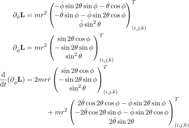
$\begin{aligned} \partial_\theta\mathbf{L} & = mr^2\begin{pmatrix} 2\dot{\phi}\cos 2\theta\cos\phi -\dot{\theta}\sin\phi \\ \dot{\theta}\cos\phi -2\dot{\phi}\cos 2\theta\sin\phi \\ 2\dot{\phi}\sin 2\theta \\ \end{pmatrix}^T_{(i,j,k)}\\ \partial_{\dot{\theta}}\mathbf{L} & = mr^2\begin{pmatrix} -\sin\phi \\ \cos\phi \\ 0 \\ \end{pmatrix}^T_{(i,j,k)} \\ \displaystyle{\frac{\mathrm{d}}{\mathrm{d}t}(\partial_{\dot{\theta}}}\mathbf{L}) & = 2mr\dot{r}\begin{pmatrix} -\sin\phi \\ \cos\phi \\ 0 \\ \end{pmatrix}^T_{(i,j,k)} + mr^2\begin{pmatrix} -\dot{\phi}\cos\phi \\ -\dot{\phi}\sin\phi \\ 0 \\ \end{pmatrix}^T_{(i,j,k)}\\ & = mr\begin{pmatrix} -2\dot{r}\sin\phi -r\dot{\phi}\cos\phi \\ 2\dot{r}\cos\phi -r\dot{\phi}\sin\phi \\ 0 \\ \end{pmatrix}^T_{(i,j,k)} \\ \end{aligned}$
In the case of $\phi$ ,
$\begin{aligned} \partial_{\phi}\mathbf{L} & = mr^2\begin{pmatrix} -\dot{\phi}\sin 2\theta\sin\phi -\dot{\theta}\cos\phi \\ -\dot{\theta}\sin\phi -\dot{\phi}\sin 2\theta\cos\phi \\ \dot{\phi}\sin^2\theta \\ \end{pmatrix}^T_{(i,j,k)}\\ \partial_{\dot{\phi}}\mathbf{L} & =mr^2\begin{pmatrix} \sin 2\theta\cos\phi \\ -\sin 2\theta\sin\phi \\ \sin^2\theta \\ \end{pmatrix}^T_{(i,j,k)}\\ \displaystyle{\frac{\mathrm{d}}{\mathrm{d}t}}(\partial_{\dot{\phi}}\mathbf{L}) & = 2mr\dot{r} \begin{pmatrix} \sin 2\theta\cos\phi \\ -\sin 2\theta\sin\phi \\ \sin^2\theta \\ \end{pmatrix}^T_{(i,j,k)} \\ & \qquad\quad +mr^2 \begin{pmatrix} 2\dot{\theta}\cos 2\theta\cos\phi -\dot{\phi}\sin 2\theta\sin\phi \\ -2\dot{\theta}\cos 2\theta\sin\phi -\dot{\phi}\sin 2\theta\cos\phi \\ 2\dot{\theta}\sin 2\theta \\ \end{pmatrix}^T_{(i,j,k)} \\ \end{aligned}$ Substitution of these partial derivatives into the formulae of generalized forces, (recall that [in Goldstein’s Classical Mechanics] the generalized force is given by)
Eq. (1-54):
$Q_i=-\displaystyle{\frac{\partial U}{\partial q_i}}+\displaystyle{\frac{\mathrm{d}}{\mathrm{d}t}\bigg( \frac{\partial U}{\partial \dot{q_i}} \bigg)}$
one can obtain:
$\begin{aligned}Q_r & =-\partial_rV-\sigma\cdot \partial_{r}\mathbf{L}+\sigma\cdot \displaystyle{\frac{\mathrm{d}}{\mathrm{d}t}}\partial_{\dot{r}}\mathbf{L}\\ & =F_r-2mr\sigma\cdot \begin{pmatrix} \dot{\phi}\sin 2\theta\cos\phi -\dot{\theta}\sin\phi \\ \dot{\theta}\cos\phi -\dot{\phi}\sin 2\theta\sin\phi \\ \dot{\phi}\sin^2\theta \\ \end{pmatrix}^T_{(i,j,k)}\\ \end{aligned}$
$\begin{aligned} Q_\theta & = -\sigma\cdot \partial_\theta\mathbf{L}+\displaystyle{\sigma\cdot \frac{\mathrm{d}}{\mathrm{d}t}(\partial_{\dot{\theta}}\mathbf{L})}\\ & = -mr\sigma \cdot \Bigg\{ r\begin{pmatrix} 2\dot{\phi}\cos 2\theta\cos\phi -\dot{\theta}\sin\phi \\ \dot{\theta}\cos\phi -2\dot{\phi}\cos 2\theta\sin\phi \\ 2\dot{\phi}\sin 2\theta \\ \end{pmatrix}- \begin{pmatrix} -2\dot{r}\sin\phi -r\dot{\phi}\cos\phi \\ 2\dot{r}\cos\phi -r\dot{\phi}\sin\phi \\ 0 \\ \end{pmatrix} \Bigg\} \\ & = -mr\sigma\cdot \begin{pmatrix} (2\cos 2\theta +1)r\dot{\phi}\cos\phi +(2\dot{r}-r\dot{\theta})\sin\phi \\ (1-2\cos 2\theta )r\dot{\phi}\sin\phi +(r\dot{\theta}-2\dot{r})\cos\phi \\ 2r\dot{\phi}\sin 2\theta \\ \end{pmatrix}^T_{(i,j,k)}\\ \end{aligned}$
$\begin{aligned} Q_\phi & = -\sigma\cdot \partial_\phi\mathbf{L}+\displaystyle{\sigma\cdot \frac{\mathrm{d}}{\mathrm{d}t}(\partial_{\dot{\phi}}\mathbf{L})}\\ & =-mr\sigma\cdot \Bigg\{ r\begin{pmatrix} -\dot{\phi}\sin 2\theta\sin\phi -\dot{\theta}\cos\phi \\ -\dot{\theta}\sin\phi -\dot{\phi}\sin 2\theta\cos\phi \\ \dot{\phi}\sin^2\theta \\ \end{pmatrix}-2\dot{r} \begin{pmatrix} \sin 2\theta\cos\phi \\ -\sin 2\theta\sin\phi \\ \sin^2\theta \\ \end{pmatrix}\\ &\qquad\quad -r \begin{pmatrix} 2\dot{\theta}\cos 2\theta\cos\phi -\dot{\phi}\sin 2\theta\sin\phi \\ -2\dot{\theta}\cos 2\theta\sin\phi -\dot{\phi}\sin 2\theta\cos\phi \\ 2\dot{\theta}\sin 2\theta \\ \end{pmatrix} \Bigg\}\\ & = -mr\sigma \cdot \begin{pmatrix} -(r\dot{\theta}+2\dot{r}\sin 2\theta +2r\dot{\theta}\cos 2\theta )\cos\phi \\ -(r\dot{\theta}+2\dot{r}\sin 2\theta +2r\dot{\theta}\cos 2\theta )\sin\phi \\ \big( (r\dot{\phi}-2\dot{r})\sin\theta -2r\dot{\theta}\cos\theta \big) \sin\theta \\ \end{pmatrix}^T_{(i,j,k)} \end{aligned}$

2.

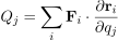
In Goldstein’s Classical Mechanics, the components of the generalized force is defined
Eq. (1.49):
$Q_j=\displaystyle{\sum_{i}\mathbf{F}_i\cdot \frac{\partial \mathbf{r}_i}{\partial q_j}}$
Hence I am to check the following three identities:
(I): $Q_r=\mathbf{F}_x\cdot \displaystyle{\frac{\partial x}{\partial r}}+\mathbf{F}_y\cdot \displaystyle{\frac{\partial y}{\partial r}}+\mathbf{F}_z\cdot \displaystyle{\frac{\partial z}{\partial r}}$ ;
(II): $Q_\theta =\mathbf{F}_x\cdot \displaystyle{\frac{\partial x}{\partial \theta}}+\mathbf{F}_y\cdot \displaystyle{\frac{\partial y}{\partial \theta}}+\mathbf{F}_z\cdot \displaystyle{\frac{\partial z}{\partial \theta}}$ ;
(III): $Q_\phi =\mathbf{F}_x\cdot \displaystyle{\frac{\partial x}{\partial \phi}}+\mathbf{F}_y\cdot \displaystyle{\frac{\partial y}{\partial \phi }}+\mathbf{F}_z\cdot \displaystyle{\frac{\partial z}{\partial \phi}}$
By abusage of notation, in what follows $Q_x$ shall replace $\mathbf{F}_x$ and be referred to as the generalized force in generalized coordinate $x$ ; and $F_x$ shall be referred to as the $x$ -component of the (usual) force $F$ due to the (usual) potential $V$ . The same notation applies likewise to $Q_y$ , $Q_z$ , $F_y$ , $F_z$ , etc.
It is convenient to check from the RHS. And let me begin with identity (I):
$\begin{aligned} \textrm{RHS} & = \begin{pmatrix} Q_x\\ Q_y \\ Q_z \\ \end{pmatrix}^T\cdot \begin{pmatrix} \displaystyle{\frac{\partial x}{\partial r}} \\ \displaystyle{\frac{\partial y}{\partial r}} \\ \displaystyle{\frac{\partial z}{\partial r}} \\ \end{pmatrix} = \begin{pmatrix} F_x+2m\sigma\cdot (0,\dot{z},-\dot{y}) \\ F_y+2m\sigma\cdot (-\dot{z},0,\dot{x}) \\ F_z+2m\sigma\cdot (\dot{y},-\dot{x},0) \\ \end{pmatrix}^T\cdot \begin{pmatrix} \displaystyle{\frac{\partial x}{\partial r}} \\ \displaystyle{\frac{\partial y}{\partial r}} \\ \displaystyle{\frac{\partial z}{\partial r}} \\ \end{pmatrix}\\ & = \displaystyle{\sum_{i=x,y,z}F_i\cdot \displaystyle{\frac{\partial r_i}{\partial r}}} + \begin{pmatrix} 2m\sigma\cdot (0,\dot{z},-\dot{y}) \\ 2m\sigma\cdot (-\dot{z},0,\dot{x}) \\ 2m\sigma\cdot (\dot{y},-\dot{x},0) \\ \end{pmatrix}^T\cdot \begin{pmatrix} \sin\theta\cos\phi \\ \sin\theta\sin\phi \\ \cos\theta \\ \end{pmatrix}\\ & =F_r + 2m\sigma\cdot \begin{pmatrix} (0,\dot{z},-\dot{y}) \\ (-\dot{z},0,\dot{x}) \\ (\dot{y},-\dot{x},0) \\ \end{pmatrix}^T\cdot \begin{pmatrix} \sin\theta\cos\phi \\ \sin\theta\sin\phi \\ \cos\theta \\ \end{pmatrix}\\ \end{aligned}$
Computing term-by-term, the first term is
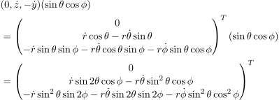
$\begin{aligned} & (0,\dot{z},-\dot{y})(\sin\theta\cos\phi) \\ & = \begin{pmatrix} 0 \\ \dot{r}\cos\theta -r\dot{\theta}\sin\theta \\ -\dot{r}\sin\theta\sin\phi -r\dot{\theta}\cos\theta\sin\phi -r\dot{\phi}\sin\theta\cos\phi \\ \end{pmatrix}^T(\sin\theta\cos\phi )\\ & = \begin{pmatrix} 0 \\ \dot{r}\sin 2\theta\cos\phi -r\dot{\theta}\sin^2\theta\cos\phi \\ -\dot{r}\sin^2\theta\sin 2\phi -r\dot{\theta}\sin 2\theta\sin 2\phi -r\dot{\phi}\sin^2\theta\cos^2\phi \\ \end{pmatrix}^T\\ \end{aligned}$
the second term is
$\begin{aligned} & (-\dot{z},0,\dot{x})(\sin\theta\sin\phi ) \\ & = \begin{pmatrix} -\dot{r}\cos\theta +r\dot{\theta}\sin\theta \\ 0\\ \dot{r}\sin\theta\cos\phi +r\dot{\theta}\cos\theta\cos\phi -r\dot{\phi}\sin\theta\sin\phi \\ \end{pmatrix}^T (\sin\theta\sin\phi ) \\ & = \begin{pmatrix} -\dot{r}\sin 2\theta\sin\phi +r\dot{\theta}\sin^2\theta\sin\phi \\ 0 \\ \dot{r}\sin^2\theta\sin 2\phi +r\dot{\theta}\sin 2\theta\sin 2\phi -r\dot{\phi}\sin^2\theta\sin^2\phi \\ \end{pmatrix}^T\\ \end{aligned}$
and the third and last term is
$\begin{aligned} & (\dot{y},-\dot{x},0)(\cos\theta )\\ & = \begin{pmatrix} \dot{r}\sin\theta\sin\phi +r\dot{\theta}\cos\theta\sin\phi +r\dot{\phi}\sin\theta\cos\phi \\ -\dot{r}\sin\theta\cos\phi -r\dot{\theta}\cos\theta\cos\phi +r\dot{\phi}\sin\theta\sin\phi \\ 0\\ \end{pmatrix}^T(\cos\theta )\\ & = \begin{pmatrix} \dot{r}\sin 2\theta\sin\phi +r\dot{\theta}\cos^2\theta\sin\phi +r\dot{\phi}\sin 2\theta\cos\phi \\ -\dot{r}\sin 2\theta\cos\phi -r\dot{\theta}\cos^2\theta\cos\phi +r\dot{\phi}\sin 2\theta \sin\phi \\ 0 \\ \end{pmatrix}^T\\ \end{aligned}$
Summing over these three terms, i.e.,
$(0,\dot{z},-\dot{y})(\sin\theta\cos\phi)+(-\dot{z},0,\dot{x})(\sin\theta\sin\phi )+(\dot{y},-\dot{x},0)(\cos\theta )$ ,
and one shall obtain from it
$\begin{pmatrix} r\dot{\theta}\sin\phi +r\dot{\phi}\sin 2\theta \cos\phi \\ r\dot{\phi}\sin 2\theta\sin\phi -r\dot{\theta}\cos\phi \\ -r\dot{\phi}\sin^2\theta \\ \end{pmatrix}^T_{(i,j,k)}$
Thus,
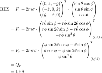
$\begin{aligned} \textrm{RHS}& = F_r + 2m\sigma\cdot \begin{pmatrix} (0,\dot{z},-\dot{y}) \\ (-\dot{z},0,\dot{x}) \\ (\dot{y},-\dot{x},0) \\ \end{pmatrix}^T\cdot \begin{pmatrix} \sin\theta\cos\phi \\ \sin\theta\sin\phi \\ \cos\theta \\ \end{pmatrix}\\ & =F_r+2m\sigma \cdot \begin{pmatrix} r\dot{\theta}\sin\phi +r\dot{\phi}\sin 2\theta \cos\phi \\ r\dot{\phi}\sin 2\theta\sin\phi -r\dot{\theta}\cos\phi \\ -r\dot{\phi}\sin^2\theta \\ \end{pmatrix}^T_{(i,j,k)}\\ & = F_r-2mr\sigma\cdot \begin{pmatrix} \dot{\phi}\sin 2\theta\cos\phi -\dot{\theta}\sin\phi \\ \dot{\theta}\cos\phi -\dot{\phi}\sin 2\theta\sin\phi \\ \dot{\phi}\sin^2\theta \\ \end{pmatrix}^T_{(i,j,k)}\\ & = Q_r \\ & = \textrm{LHS}\\ \end{aligned}$
The identity (I) is checked.
By applying the same procedure one can easily check that identities (II) and (III) are also satisfied. This is left as a tedious exercise to the reader. And the components of (generalized/usual) force in two coordinates systems are indeed related to each other as
Eq. (1.49):

$Q_j=\displaystyle{\sum_{i}\mathbf{F}_i\cdot \frac{\partial \mathbf{r}_i}{\partial q_j}}$

3.

In this part I shall obtain the equation of motion, or the Euler-Lagrange equations, where the Lagrangian $\mathcal{L}$ is defined to be the difference of kinetic energy and generalized potential, i.e., $\mathcal{L}=T-U$ .
To begin with, I shall show that owing to its linearity, the Lagrangian is separable in the sense of the following:
$\begin{aligned} \displaystyle{\frac{\mathrm{d}}{\mathrm{d}t}\bigg( \frac{\partial \mathcal{L}}{\partial \dot{q_i}} \bigg)}-\displaystyle{\frac{\partial \mathcal{L}}{\partial q_i}} & =0\\ \displaystyle{\frac{\mathrm{d}}{\mathrm{d}t}\bigg( \frac{\partial}{\partial \dot{q_i}}\big( T-U \big)\ \bigg)}-\displaystyle{\frac{\partial }{\partial q_i}}\big( T-U \big) & =0\\ \displaystyle{\frac{\mathrm{d}}{\mathrm{d}t}\bigg( \frac{\partial}{\partial \dot{q_i}}\big( T \big) - \frac{\partial}{\partial \dot{q_i}}\big( U \big) \bigg)}-\displaystyle{\frac{\partial }{\partial q_i}}\big( T \big) + \displaystyle{ \frac{\partial }{\partial q_i}}\big( U \big) & =0\\ \displaystyle{\frac{\mathrm{d}}{\mathrm{d}t}\bigg( \frac{\partial}{\partial \dot{q_i}}\big( T \big) \bigg)}-\displaystyle{\frac{\partial }{\partial q_i}}\big( T \big) & =\displaystyle{\frac{\mathrm{d}}{\mathrm{d}t}\bigg( \frac{\partial}{\partial \dot{q_i}}\big( U \big) \bigg)} - \displaystyle{ \frac{\partial }{\partial q_i}}\big( U \big) \\ \displaystyle{\frac{\mathrm{d}}{\mathrm{d}t}\bigg( \frac{\partial}{\partial \dot{q_i}}\big( T \big) \bigg)}-\displaystyle{\frac{\partial }{\partial q_i}}\big( T \big) & =Q_i \\ \end{aligned}$
where $Q_i$ is the generalized force defined in the previous parts (a) & (b).
Based on the transformation equation of velocity between spherical and Cartesian coordinates as derived in part (a):
$\begin{aligned} \mathbf{v} & =(\dot{x},\dot{y},\dot{z})\\ & = \begin{pmatrix} \dot{r}\sin\theta\cos\phi +r\dot{\theta}\cos\theta\cos\phi -r\dot{\phi}\sin\theta\sin\phi \\ \dot{r}\sin\theta\sin\phi +r\dot{\theta}\cos\theta\sin\phi +r\dot{\phi}\sin\theta\cos\phi \\ \dot{r}\cos\theta -r\dot{\theta}\sin\theta \\ \end{pmatrix}^T_{(i,j,k)}\\ \end{aligned}$ ,
the conversion of kinetic energy $T$ into spherical coordinates can be derived in the form:
$\begin{aligned} T & =\displaystyle{\frac{1}{2}m\mathbf{v}^2=\frac{1}{2}m(\dot{x}^2+\dot{y}^2+\dot{z}^2)}\\ & = \cdots \\ & = \displaystyle{\frac{1}{2}mr^2(\dot{\theta}^2+\sin^2\theta \dot{\phi}^2)} \\\end{aligned}$
That said, I shall compute the following derivatives:
$\displaystyle{\frac{\partial T}{\partial r}}=mr(\dot{\theta}^2+\sin^2\theta\dot{\phi}^2)$ , $\displaystyle{\frac{\partial T}{\partial \dot{r}}}=0$ , $\displaystyle{\frac{\mathrm{d}}{\mathrm{d}t}\bigg(\frac{\partial T}{\partial \dot{r}}\bigg)}=0$
$\displaystyle{\frac{\partial T}{\partial \theta}}=mr^2\dot{\phi}^2\sin 2\theta$ , $\displaystyle{\frac{\partial T}{\partial \dot{\theta}}}=mr^2\dot{\theta}$ , $\displaystyle{\frac{\mathrm{d}}{\mathrm{d}t}\bigg(\frac{\partial T}{\partial \dot{\theta}}\bigg)}=mr^2\ddot{\theta}+2m\dot{\theta}r\dot{r}$
$\displaystyle{\frac{\partial T}{\partial \phi}}=0$ , $\displaystyle{\frac{\partial T}{\partial \dot{\phi}}}=mr^2\dot{\phi}$ , $\displaystyle{\frac{\mathrm{d}}{\mathrm{d}t}\bigg(\frac{\partial T}{\partial \dot{\phi}}\bigg)}=mr^2\ddot{\phi}+2m\dot{\phi}r\dot{r}$
Thus, the LHS of the separable Lagrangian equations are
$\begin{aligned}\widetilde{T}_r & =-mr(\dot{\theta}^2+\sin^2\theta\dot{\phi}^2)\\ \widetilde{T}_\theta & =mr^2\ddot{\theta}+2m\dot{\theta}r\dot{r}-mr^2\dot{\phi}^2\sin 2\theta \\ \widetilde{T}_\phi & =mr^2\ddot{\phi}+2m\dot{\phi}r\dot{r}\end{aligned}$
Equating them with the $Q_r$ , $Q_\theta$ , and $Q_\phi$ which were derived in part (a), we obtain three equations of motion:
$-mr(\dot{\theta}^2+\sin^2\theta\dot{\phi}^2)=F_r-2mr\sigma\cdot \begin{pmatrix} \dot{\phi}\sin 2\theta\cos\phi -\dot{\theta}\sin\phi \\ \dot{\theta}\cos\phi -\dot{\phi}\sin 2\theta\sin\phi \\ \dot{\phi}\sin^2\theta \\ \end{pmatrix}^T_{(i,j,k)}$
$mr^2\ddot{\theta}+2m\dot{\theta}r\dot{r}-mr^2\dot{\phi}^2\sin 2\theta = -mr\sigma\cdot \begin{pmatrix} (2\cos 2\theta +1)r\dot{\phi}\cos\phi +(2\dot{r}-r\dot{\theta})\sin\phi \\ (1-2\cos 2\theta )r\dot{\phi}\sin\phi +(r\dot{\theta}-2\dot{r})\cos\phi \\ 2r\dot{\phi}\sin 2\theta \\ \end{pmatrix}^T_{(i,j,k)}$
$mr^2\ddot{\phi}+2m\dot{\phi}r\dot{r} =-mr\sigma \cdot \begin{pmatrix} -(r\dot{\theta}+2\dot{r}\sin 2\theta +2r\dot{\theta}\cos 2\theta )\cos\phi \\ -(r\dot{\theta}+2\dot{r}\sin 2\theta +2r\dot{\theta}\cos 2\theta )\sin\phi \\ \big( (r\dot{\phi}-2\dot{r})\sin\theta -2r\dot{\theta}\cos\theta \big) \sin\theta \\ \end{pmatrix}^T_{(i,j,k)}$

Remark.

The in the first equation of motion is the central force. The fixed vector should be in component form . Once having dotted with the rightmost row vector, a scalar will be obtained.

November 19, 2019October 25, 2022

201911190336 Homework 1, Differential Geometry

Let $\boldsymbol{\alpha} :I\rightarrow \mathbb{R}^3$ be a regular parametrized curve (not necessarily by arc length) and let $\beta :J\rightarrow \mathbb{R}^3$ be a reparametrization of $\boldsymbol{\alpha}$ by the arc length $s=s(t)$ measured from $t_0\in I$ .

Let also $t=t(s)$ be the inverse function of $s$ and denote the derivative of $\boldsymbol{\alpha}$ wrt $t$ by $\boldsymbol{\alpha}'$ . Prove that

i. $\mathrm{d}t/ \mathrm{d}s=1/\|\boldsymbol{\alpha}'\|$ and $\mathrm{d}^2t/ \mathrm{d}s^2=-\langle \boldsymbol{\alpha}',\boldsymbol{\alpha}''\rangle /\|\boldsymbol{\alpha}'\|^4$ ;

ii. The curvature of $\boldsymbol{\alpha}$ at $t\in I$ is $\kappa (t)=\displaystyle{\frac{\|\boldsymbol{\alpha}' \wedge\boldsymbol{\alpha}''\|}{\|\boldsymbol{\alpha}'\|^3}}$ ; and

iii. The torsion of $\boldsymbol{\alpha}$ at $t\in I$ is $\tau (t)=\displaystyle{-\frac{\langle \boldsymbol{\alpha}' \wedge \boldsymbol{\alpha}'',\boldsymbol{\alpha}'''\rangle }{\| \boldsymbol{\alpha}' \wedge\boldsymbol{\alpha}''\|^2}}$ .

Solution.

i. By definition $\displaystyle{\frac{\mathrm{d}\boldsymbol{\alpha}}{\mathrm{d}t}}=\boldsymbol{\alpha}'$ .

Using chain rule,

$\displaystyle{\frac{\mathrm{d}\boldsymbol{\alpha}}{\mathrm{d}t}}= \displaystyle{\frac{\mathrm{d}\boldsymbol{\alpha}}{\mathrm{d}s}}\displaystyle{\frac{\mathrm{d}s}{\mathrm{d}t}}$ .

After taking the norm, as a consequence of natural parametrization

(i.e., $\bigg| \displaystyle{\frac{\mathrm{d}\boldsymbol{\alpha}}{\mathrm{d}s}}\bigg| =1$ ),

we have

$\| \boldsymbol{\alpha}'\|=\bigg| \displaystyle{\frac{\mathrm{d}\boldsymbol{\alpha}}{\mathrm{d}s}} \bigg| \bigg| \displaystyle{\frac{\mathrm{d}s}{\mathrm{d}t}} \bigg|= \bigg| \displaystyle{\frac{\mathrm{d}s}{\mathrm{d}t}}\bigg|$ .

Hence $\mathrm{d}t/\mathrm{d}s=1/ \| \boldsymbol{\alpha}'\|$ .

That said,

$\begin{aligned} \displaystyle{\frac{\mathrm{d}^2t}{\mathrm{d}s^2}} & =\bigg( \displaystyle{\frac{\mathrm{d}t}{\mathrm{d}s}} \bigg) \displaystyle{\frac{\mathrm{d}}{\mathrm{d}t}}\bigg( \displaystyle{\frac{\mathrm{d}t}{\mathrm{d}s}} \bigg) \\ & =\displaystyle{\frac{1}{\| \boldsymbol{\alpha}' \|}}\frac{\mathrm{d}}{\mathrm{d}t}\bigg(\displaystyle{\frac{1}{\|\boldsymbol{\alpha}' \|}}\bigg) \\ & =\displaystyle{\frac{1}{\| \boldsymbol{\alpha}' \|}}\frac{\mathrm{d}}{\mathrm{d}t}\bigg(\displaystyle{\frac{1}{\langle \boldsymbol{\alpha}',\boldsymbol{\alpha}' \rangle^{1/2}}}\bigg)\\ \end{aligned}$ .

But,

$\begin{aligned} & \displaystyle{\frac{\mathrm{d}}{\mathrm{d}t}}\bigg(\displaystyle{\frac{1}{\langle \boldsymbol{\alpha}',\boldsymbol{\alpha}' \rangle^{1/2}}}\bigg)\\ & =-\displaystyle{\frac{1}{2}}\langle \boldsymbol{\alpha}',\boldsymbol{\alpha}' \rangle^{-3/2}\Big( \langle \boldsymbol{\alpha}',\boldsymbol{\alpha}'' \rangle +\langle \boldsymbol{\alpha}'',\boldsymbol{\alpha}' \rangle \Big) \\ & =-\langle \boldsymbol{\alpha}',\boldsymbol{\alpha}' \rangle^{-3/2}\langle \boldsymbol{\alpha}',\boldsymbol{\alpha}'' \rangle \\ \end{aligned}$ .

Thus,

$\begin{aligned} \displaystyle{\frac{\mathrm{d}^2t}{\mathrm{d}s^2}} & =-\displaystyle{\frac{1}{\| \boldsymbol{\alpha}' \|}}\langle \boldsymbol{\alpha}',\boldsymbol{\alpha}' \rangle^{-3/2}\langle \boldsymbol{\alpha}',\boldsymbol{\alpha}'' \rangle \\ & =-\displaystyle{\frac{1}{\langle \boldsymbol{\alpha}',\boldsymbol{\alpha}' \rangle^{1/2}}}\langle \boldsymbol{\alpha}',\boldsymbol{\alpha}' \rangle^{-3/2}\langle \boldsymbol{\alpha}',\boldsymbol{\alpha}'' \rangle \\ & = \displaystyle{-\frac{\langle \boldsymbol{\alpha}',\boldsymbol{\alpha}'' \rangle}{\big( \langle \boldsymbol{\alpha}', \boldsymbol{\alpha}'\rangle^{1/2}\big)^4}} \\ & =-\langle \boldsymbol{\alpha}',\boldsymbol{\alpha}''\rangle /\|\boldsymbol{\alpha}'\|^4 \\ \end{aligned}$ .

ii.

$\boldsymbol{\alpha}'= \displaystyle{\frac{\mathrm{d}\boldsymbol{\alpha}}{\mathrm{d}t}}=\displaystyle{\frac{\mathrm{d}\boldsymbol{\alpha}}{\mathrm{d}s}}\displaystyle{\frac{\mathrm{d}s}{\mathrm{d}t}}=\dot{\boldsymbol{\alpha}}s'$ .

Besides,

$\boldsymbol{\alpha}''=\displaystyle{\frac{\mathrm{d}}{\mathrm{d}t}}(\dot{\boldsymbol{\alpha}}s')=\dot{\boldsymbol{\alpha}}\displaystyle{\frac{\mathrm{d}s'}{\mathrm{d}t}}+s'\displaystyle{\frac{\mathrm{d}\dot{\boldsymbol{\alpha}}}{\mathrm{d}t}}=\dot{\boldsymbol{\alpha}}s''+(s')^2\ddot{\boldsymbol{\alpha}}$ .

Then,

$\langle \boldsymbol{\alpha}'\wedge \boldsymbol{\alpha}'' \rangle =\big( \dot{\boldsymbol{\alpha}}s' \big) \times \big( \dot{\boldsymbol{\alpha}}s''+(s')^2\ddot{\boldsymbol{\alpha}} \big) =(s')^3\langle\dot{\boldsymbol{\alpha}}\wedge \ddot{\boldsymbol{\alpha}} \rangle =\|\boldsymbol{\alpha}'\|^3 \langle \dot{\boldsymbol{\alpha}}\wedge \ddot{\boldsymbol{\alpha}} \rangle$ .

(For $\mathrm{d}s/\mathrm{d}t=\| \boldsymbol{\alpha}'\|$ of part i. is used.)

It follows that

$\langle \boldsymbol{\alpha}'\wedge \boldsymbol{\alpha}'' \rangle =\|\boldsymbol{\alpha}\|^3 \| \dot{\boldsymbol{\alpha}} \|\| \ddot{\boldsymbol{\alpha}}\|\sin \measuredangle (\dot{\boldsymbol{\alpha}},\ddot{\boldsymbol{\alpha}})$ .

Note that $\dot{\boldsymbol{\alpha}}=\mathbf{t}$ and $\ddot{\boldsymbol{\alpha}}=\dot{t}$ are orthogonal,

$\| \boldsymbol{\alpha}\|=1$ and $\| \ddot{\boldsymbol{\alpha}}\|=\| \dot{\mathbf{t}}\|=\| \kappa\|$ .

We obtain

$\kappa (t)=\displaystyle{\frac{\|\boldsymbol{\alpha}' \wedge\boldsymbol{\alpha}''\|}{\|\boldsymbol{\alpha}'\|^3}}$ .

iii.

First,

$\dot{\boldsymbol{\alpha}}=\displaystyle{\frac{\mathrm{d}\boldsymbol{\alpha}}{\mathrm{d}s}}=\displaystyle{\frac{\mathrm{d}\boldsymbol{\alpha}}{\mathrm{d}t}}\displaystyle{\frac{\mathrm{d}t}{\mathrm{d}s}}=\boldsymbol{\alpha}'\dot{t}$ ;

secondly,

$\ddot{\boldsymbol{\alpha}}=\displaystyle{\frac{\mathrm{d}}{\mathrm{d}s}}(\boldsymbol{\alpha}'\dot{t})=\boldsymbol{\alpha}'\ddot{t}+\bigg( \displaystyle{\frac{\mathrm{d}}{\mathrm{d}s}}\boldsymbol{\alpha}' \bigg)\dot{t}=\boldsymbol{\alpha}'\ddot{t}+\boldsymbol{\alpha}''\dot{t}^2$ ;

thirdly,

$\dddot{\boldsymbol{\alpha}}=\displaystyle{\frac{\mathrm{d}}{\mathrm{d}s}}\big( \boldsymbol{\alpha}'\ddot{t}+\boldsymbol{\alpha}''\dot{t}^2 \big) =\boldsymbol{\alpha}'\dddot{t}+\boldsymbol{\alpha}''\dot{t}\ddot{t}+\boldsymbol{\alpha}''2\dot{t}\ddot{t}+\boldsymbol{\alpha}'''\dot{t}^3=\boldsymbol{\alpha}'\dddot{t}+2\boldsymbol{\alpha}''\dot{t}\ddot{t}+\boldsymbol{\alpha}'''\dot{t}^3$ .

Compute $\langle \dot{\boldsymbol{\alpha}}\wedge \ddot{\boldsymbol{\alpha}}, \dddot{\boldsymbol{\alpha}} \rangle$ as follows:

$\begin{aligned} \langle \dot{\boldsymbol{\alpha}}\wedge \ddot{\boldsymbol{\alpha}}, \dddot{\boldsymbol{\alpha}} \rangle & = \big( \boldsymbol{\alpha}'\dot{t} \big) \wedge \big( \boldsymbol{\alpha}'\ddot{t}+\boldsymbol{\alpha}''\dot{t}^2 \big) \cdot \big( \boldsymbol{\alpha}'\dddot{t}+2\boldsymbol{\alpha}''\dot{t}\ddot{t}+\boldsymbol{\alpha}'''\dot{t}^3 \big) \\ & =\big( \boldsymbol{\alpha}'\dot{t}\wedge \boldsymbol{\alpha}''\dot{t}^2\big) \cdot \big( \boldsymbol{\alpha}'\dddot{t}+2\boldsymbol{\alpha}''\dot{t}\ddot{t}+\boldsymbol{\alpha}'''\dot{t}^3 \big)\\ \end{aligned}$

Now that the cross product $\boldsymbol{\alpha}'\wedge \boldsymbol{\alpha}''$ is orthogonal to both $\boldsymbol{\alpha}'$ and $\boldsymbol{\alpha}''$ , we can ignore the dot product among them and what remains is

$(\boldsymbol{\alpha}'\dot{t}\wedge \boldsymbol{\alpha}''\dot{t}^2)\cdot \boldsymbol{\alpha}'''\dot{t}^3$ , or,

$\dot{t}^6\langle \boldsymbol{\alpha}'\wedge \boldsymbol{\alpha}'', \boldsymbol{\alpha}'''\rangle$ .

Using the result of part i., substitute $1/\| \boldsymbol{\alpha}'\|$ for $\dot{t}$ , we obtain

$\langle \dot{\boldsymbol{\alpha}}\wedge \ddot{\boldsymbol{\alpha}}, \dddot{\boldsymbol{\alpha}} \rangle=\displaystyle{\frac{\langle \boldsymbol{\alpha}'\wedge \boldsymbol{\alpha}'', \boldsymbol{\alpha}'''\rangle}{\|\boldsymbol{\alpha}'\|^6}}$ .

Using the formula for curvature in part ii. and put it into

$\tau =\displaystyle{\frac{\langle \dot{\boldsymbol{\alpha}}\wedge \ddot{\boldsymbol{\alpha}},\dddot{\boldsymbol{\alpha}} \rangle}{\kappa^2}}=\displaystyle{\frac{\langle \boldsymbol{\alpha}'\wedge \boldsymbol{\alpha}'', \boldsymbol{\alpha}'''\rangle}{\kappa^2 \|\boldsymbol{\alpha}'\|^6}}$ ,

i.e.,

$\tau (t)=\displaystyle{-\frac{\langle \boldsymbol{\alpha}' \wedge \boldsymbol{\alpha}'',\boldsymbol{\alpha}'''\rangle }{\| \boldsymbol{\alpha}' \wedge\boldsymbol{\alpha}''\|^2}}$ .

November 18, 2019October 24, 2022

201911181237 Example 1.1

Put the equations of the circular helix (3) in the form (8).

Background.

Eq. (3):

$x=a\cos u$ , $y=a\sin u$ , $z=bu$

is the parametric form of a circular helix.

Eq. (8):

$x=x$ , $y=F_2(x)$ , $z=F_3(x)$

is another form of the equations of a curve.

Let $x\stackrel{\mathrm{def}}{=} a\cos u$ ,

or $u=\displaystyle{\cos^{-1}\bigg( \frac{x}{a} \bigg)}$ .

$\begin{aligned} x^2 & = a^2\cos^2 u \\ a^2 - x^2 & = a^2 - a^2 \cos^2 u = a^2\sin^2 u \\ \pm \sqrt{a^2-x^2} & = a\sin u \\ y & = \pm \sqrt{a^2-x^2} \end{aligned}$

$z=b\cos^{-1}\displaystyle{\bigg( \frac{x}{a} \bigg)}$ .

In sum, the circular helix is now expressed in the form

$\begin{aligned} x & = a\cos u \\ y & = F_2(x)=\pm\sqrt{a^2-x^2} \\ z & =F_3(x)=b\cos^{-1}\bigg( \frac{x}{a} \bigg) \\ \end{aligned}$

Remark. In this form the curve is really defined by the last two equations, or, if it be a plane curve in the $xy$ -plane, its equation is in the customary form Eq. (9): $y=f(x)$ .

_{pg.3 , Chapter 1 Curves in Space}

CASE 1: Would it be possible that ?

CASE 2: If for all elements in the group , their order cannot ever be .

CASE I of Mercury

CASE II of Venus

CASE 1: Would it be possible that $a=e$ ?

CASE 2: If for all elements in the group $G$ , their order cannot ever be $2$ .