Solve the following equations:
(a)  .
.
(b)  .
.
(c)  .
.
(d)  .
.
(e) ![\displaystyle{\frac{1}{4}(3y-2)-\bigg[ y-\frac{1}{y}(7-3y)\bigg] =-\frac{1}{4}y-7}](https://physicspupil.com/wp-content/ql-cache/quicklatex.com-fc95addad543512317800f8a23bd4507_l3.svg "Rendered by QuickLaTeX.com") .
.
Extracted from K. L. Nielsen. (1958). College Mathematics.
Roughwork.
(a)

(b)
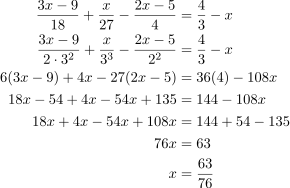
(c)
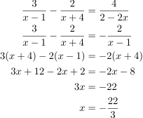
(d) Not to be attempted.
(e) Not to be attempted.

物理子衿
Solve the following equations:
(a) .
(b) .
(c) .
(d) .
(e) .
Extracted from K. L. Nielsen. (1958). College Mathematics.
Roughwork.
(a)
(b)
(c)
(d) Not to be attempted.
(e) Not to be attempted.
Solve these simultaneous equations:
1. 
Roughwork. Read More
Substituting  for
for  :
:
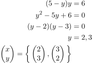
2. 
Roughwork. Read More
Substituting  for :
for :

3. 
Roughwork. Read More
Substituting  for
for  :
:
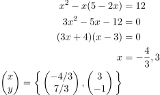
4. 
Roughwork. Read More
Substituting  for :
for :

5. 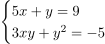
Roughwork. Read More
Substituting  for :
for :
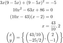
6. 
Roughwork. Read More
Substituting  for :
for :

7. 
Roughwork. Read More
Substituting  for :
for :
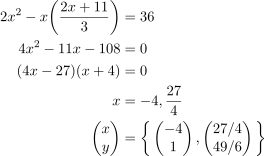
8. 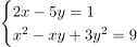
Roughwork. Read More
Substituting  for :
for :

9. 
Roughwork. Read More
Substituting  for :
for :

10. 
Roughwork. Read More
Substituting  for :
for :
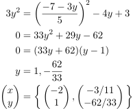
Extracted from A. Godman & J. F. Talbert. (1975). Additional Mathematics Pure and Applied in SI Units.
This problem is not to be attempted.
(A001) Scalar ( ). A quantity with magnitude only. Read More
 in metre
  , mass
  in kilogram
  , time
  in second
  , temperature
  in Kelvin
  , electric current
  in Ampere
  , amount of substance
  in mole
  , and light intensity
  in candela
  , of dimensions
 ![[L]](https://physicspupil.com/wp-content/ql-cache/quicklatex.com-283f010575e7faea78d89561d3b25462_l3.svg "Rendered by QuickLaTeX.com") ,
, ![[M]](https://physicspupil.com/wp-content/ql-cache/quicklatex.com-41efb3cdc699b51e117b827dd2b2532a_l3.svg "Rendered by QuickLaTeX.com") ,
, ![[T]](https://physicspupil.com/wp-content/ql-cache/quicklatex.com-b046b88ef5231f9f99b3921141fb931a_l3.svg "Rendered by QuickLaTeX.com") ,
, ![[\Theta]](https://physicspupil.com/wp-content/ql-cache/quicklatex.com-f436b30f65df4d1ff66c13c795242a6b_l3.svg "Rendered by QuickLaTeX.com") ,
, ![[I]](https://physicspupil.com/wp-content/ql-cache/quicklatex.com-e620fa48094760bf56e357e8b427a43e_l3.svg "Rendered by QuickLaTeX.com") ,
, ![[N]](https://physicspupil.com/wp-content/ql-cache/quicklatex.com-29a0c2bc4a1dac7e822a44dbb7354ec4_l3.svg "Rendered by QuickLaTeX.com") , and
, and ![[J]](https://physicspupil.com/wp-content/ql-cache/quicklatex.com-6010a8c42b968acaf68f251160a6b246_l3.svg "Rendered by QuickLaTeX.com") .
. (A002) Vector ( ,
,  ). A quantity with magnitude (size) and direction. Read More
 of magnitude
  ; ii. displacement
  (change in position)
  ; iii. average velocity
  during time interval
  ; iv. instantaneous velocity
  of magnitude
  the speed; v. average acceleration
  ; and vi. instantaneous acceleration
  .
. (A003) Distance. How far something travels, a scalar. Read More
 , in dimension of length .
(A004) Displacement (,  ). How far something travels in a given direction, a vector. Read More
, its magnitude  being a scalar. Path-independent. Its SI unit is metre, , in dimension of length .
(A005) Speed. How fast something is moving, a scalar. Read More
 . Its SI unit is
  , in dimensions
 ![\displaystyle{\frac{[L]}{[T]}}](https://physicspupil.com/wp-content/ql-cache/quicklatex.com-324985ff2512d537ce90930a056ea051_l3.svg "Rendered by QuickLaTeX.com") .
.(A006) Velocity (, ). How fast something is moving in a given direction, a vector. Read More
is the change of displacement with respect to time  rate of change of displacement rate of change of distance moved in a given direction, a vector denoted by . Its unit being
  , in dimensions , and its magnitude a scalar.

(A007) Acceleration ( ,
,  ). The rate at which the velocity changes during a given amount of time, a vector denoted by . Read More
Its unit being  in dimensions
 ![\displaystyle{\frac{[L]}{[T]^2}}](https://physicspupil.com/wp-content/ql-cache/quicklatex.com-b901eca055255bb1632c377d49bf7e04_l3.svg "Rendered by QuickLaTeX.com") and its magnitude
and its magnitude  a scalar,
(A008) Free Fall. The movement of an object in response to a gravitational attraction.
(A009) Projectile. An object that moves through space acted upon only by the Earth’s gravity.
(A010) Rectilinear Motion. ( straight-line, one-dimensional, axial) Read More
For uniformly accelerated motion, i.e.,  , the equations of rectilinear motion are

(A011) Curvilinear Motion. ( parabolic, projectile, planar) Read More
For uniformly accelerated motion, i.e., , the equations of curvilinear motion are

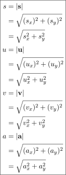
where

such that
(A012) Rotational Motion. ( uniform circular, orbital, planetary) Read More
 are
are  ,
,  , and
, and  , herein the variables being angular displacement
  , angular velocity
  , and time .


Circular motion examples. Aircraft turning a flight, vehicles rounding bends with or without banking, loop motion, satellite orbits, centrifuge, etc.
(A013) Periodic Motion. ( simple harmonic, pendulum, oscillating) Read More
Periodic motion is motion repeated in equal time interval, period. Oscillation is the back-and-forth motion about a fixed point called the equilibrium position, e.g., simple, compound, or torsion pendulum, spring-mass, and alternating current. If there is no damping force disturbing the body, it oscillates forever at the natural frequency  that is characteristic of the system. If a system whose acceleration is in magnitude proportional to displacement , and yet in opposite direction to it, i.e.,
  and
and  , it is said to be in a simple harmonic motion.
Hooke’s law states that the restoring force  is proportional to the displacement from its equilibrium position:

(A014) Force (). A push or a pull, vector denoted by  . Read More
Its magnitude being a scalar  , the unit being Newton
  , or
, or  , in dimensions
 ![\displaystyle{\frac{[M][L]}{[T]^2}}](https://physicspupil.com/wp-content/ql-cache/quicklatex.com-62c3dc5c0b846df6e0728b8ea1d50fdb_l3.svg "Rendered by QuickLaTeX.com") . E.g., gravitational force, electromagnetic force, frictional force, viscous force, upthrust, etc. The properties of force are implicitly stated in Newton’s Laws of Motion:
. E.g., gravitational force, electromagnetic force, frictional force, viscous force, upthrust, etc. The properties of force are implicitly stated in Newton’s Laws of Motion:


(A015) Friction (). The force that acts to oppose the motion between two materials moving past each other. Read More
Static (resp. kinetic) friction  is given by
  (resp.
  ). By definition, friction
  is
is  dependent on the material properties (
 ) of contact surfaces and the normal reaction (),
  independent of the speed () of motion and the area (
 ) of contact.
(A016) Static Friction ( ). The resistance force that must be overcome to start an object in motion, a vector. Read More
 with where
  is the coefficient of static friction and the normal force. The direction being which that is parallel to surface of contact, and opposes relative motion.
When net force  the object will not move. But if net force
  it will be moved.
(A017) Kinetic Friction ( ). The resistance force between two surfaces already in motion, a vector. Read More
 where
where  is the coefficient of kinetic friction and the normal force. The direction being which that is parallel to the surface of contact, and opposes relative motion.
 (A018) Statics.The study of forces in equilibrium, i.e.,  rotation acceleration. Read More
For static equilibrium, i. the net force acting on the object must be zero, i.e.,  ,
,  , and
, and  ; and ii. the net torque acting on the object must be zero
  .
.
A couple, torque, or moment of force satisfies  ii. i.
(A019) Dynamics. The study of cause and effect of motions, namely, of the agent force (contact) and the field force (non-contact).
(A020) Kinematics. The study of motions proper to the movements, being concerned with displacement  , velocity
  , acceleration
  and time only, without reference to force or mass .
(A021) Pressure. The force per unit area. Read More
Cf. Archimedes’s principle, Pascal’s principle, Bernoulli’s principle, and Stokes’s law.
(A022) Momentum ( ,
,  ). A measure of how difficult it is to stop a moving object, aka “quantity of motion” by Newton, a vector. Read More
The product of mass (aka quantity of matter) and velocity.
(A023) Impulse ( ,
,  ,
,  ,
,  ,
,  ). The product of the force exerted on an object and the time interval during which it acts, or, in essence, the change in momentum. Impulse is a vector. Read More
 . Its unit being
  or
or  .
.(A024) Elastic Collision. A collision in which objects collide and bounce apart with no energy loss. Read More
 kinetic energy are conserved.
 ;
; 
You might wish to further know of Newton’s law of restitution:

For two bodies impinging directly or obliquely, their relative velocity (wrt to one) after impact is equal to  times that before impact in the opposite direction, the constant
 ![e\in [0,1]](https://physicspupil.com/wp-content/ql-cache/quicklatex.com-87579a900046e13094ea325496e31673_l3.svg "Rendered by QuickLaTeX.com") being the coefficient of restitution ranging from
being the coefficient of restitution ranging from  (perfectly inelastic) to
  (perfectly elastic).
(A025) Inelastic Collision. A collision in which objects collide and some mechanical energy is transformed into thermal energy. Read More
 momentum, kinetic energy, is conserved.


Perfectly inelastic collision in addition is such that the colliding objects stick together after they hit each other.


Super inelastic collision as an aside is such that one object explodes into granules gaining kinetic energy by losing potential energy.


Nevertheless, in the absence of external force,  energy of a closed system is conserved, as stated by the law of conservation of energy.
(A026) Work ( ). The product of the component of the force exerted on an object in the direction of displacement and the magnitude of the displacement, a scalar. Read More

(A027) Power ( ).The rate at which work is done. Read More
Generally,  ; for mechanical power,
  ; and for power in a circuit,
(A028) Energy ( ). The ability to do work.
(A029) Potential Energy ( ,
,  ,
,  ,
,  ). Energy of position, or stored energy. Read More

(A030) Kinetic Energy ( ,
,  , ). Energy of motion. Read More

(A031) Machine. A device that helps to do work by changing the magnitude or direction of the applied force. E.g., lever, pulley, and incline.
(A032) Efficiency. The ratio of the work output to the work input.
(A033) Period (). The time it takes for one full rotation or revolution of an object, and also the time it takes for a vibrating object to repeat its motion. Read More

(A034) Frequency (). The number of rotations or revolutions per unit time, and also the number of vibrations made per unit time. Read More

(A035) Torque ( ,
,  ). A measurement of the tendency of a force to produce a rotation about an axis. Read More
Torque is the moment of force, e.g.  , where
  is the perpendicular distance of a point, say
  , from .
(A036) Center of Gravity ( ). The point on any object that acts like the place at which all the weight is concentrated.
(A037) Moment of Inertia (). The resistance of an object to changes in its rotational motion.
(A038) Angular Momentum ( ). The measure of how difficult it is to stop a rotating object, a (pseudo-)vector. Read More
Angular momentum is defined the moment of momentum, e.g.,  , where is the perpendicular distance of a point, say , from .
(A039) Law of Universal Gravitation. Every particle attracts every other particle with a force that is proportional to the mass of the particles and inversely proportional to the square of the distance between them. Read More
I.e.,  where
where  is the universal gravitational constant.
(A040) Escape Speed. The minimum speed an object must possess in order to escape from the gravitational pull of a body. Read More


(A041) Density ( ). A measure of how much mass occupies a given space. Read More

(A042) Stress. The force exerted on an area divided by the area. Read More

Its unit is either  or
or  .
.
(A043) Strain. The ratio of change in dimension to original dimension. Read More

It has no unit.
(A044) Temperature. A quantity that you can measure with a thermometer. Read More
Cf. average kinetic energy,  .
.
(A045) Heat ( ). The transfer of energy between two objects that differ in temperature. Read More
For energy transfer by conduction, the rate is given by

(A046) Specific Heat. A measure of the amount of heat needed to raise the temperature of  of a substance by
  . Read More

(A047) Latent Heat of Fusion. The quantity of heat needed per kilogram to melt a solid (or solidify a liquid) at a constant temperature and atmospheric pressure. Read More

(A048) Latent Heat of Vaporization. The quantity of heat needed per kilogram to vaporize a liquid (or liquidize a gas) at a constant temperature and atmospheric pressure. Read More

(A049) Doppler Effect. A change in the apparent frequency of sound due to the motion of the source () or the observer ( ). Read More

(A050) Reflection. The bouncing of light. Read More

(A051) Mirror/Thin Lens Equation. Read More

(A052) Wave Equation. Read More

where  is the angular wave number,
  the frequency, and
  the phase angle.
(A053) Refraction. The change in direction of light due to a change in speed as it passes from one medium to another. Read More

(A054) Diffraction. The spreading of a wave as it passes around an obstacle or through an opening. Read More
The diffraction grating equation is
 .
.
(A055) Interference. When two waves overlap to produce one new wave. Read More
Cf. constructive (/superposition) as light fringes and increased intensity of sound; destructive (/neutralization) as dark fringes and silence.
Fringe separation in double-slit interference is given by
 .
.
(A056) Electrostatics. The study of electric charges at rest, electric forces in equilibrium, and electric field under invariance.
(A057) Coulomb’s Law. Two charged objects attract each other with a force that is proportional to the charge on the objects and inversely proportional to the square of the distance between them. Read More

(A058) Electric Field. An area of influence around a charged object. The magnitude of the field is proportional to the amount of electrical force exerted on a positive test charge placed at a given point in the field. Read More
Electric field strength due to a point charge:

Electric field between parallel plates:

(A059) Potential Difference. The work done to move a test charge (resp. mass) from one location to another, denoted by  (resp.
  ).
).
(A060) Current (). The amount of charge that passes through an area in a given amount of time. Read More

Current flows from point to point  iff
iff  .
.
(A061) Resistance ( ). An opposition to the flow of charge. Read More

(A062) Capacitor. A device that stores charge on conductors that are separated by an insulator. Read More
The capacitance  of a capacitor is defined the amount of electric charges stored per unit volt .

Its unit being  or Farad (
 ).
).
(A063) Inductor. A device that stores energy to oppose the current flowing through it. Read More

(A064) Kirchhoff’s Laws. Read More
Voltage (/loop) rule: The algebraic sum of the changes in potential encountered in a complete traversal of any loop of a circuit must be zero. I.e., 
Current (/junction) rule: The sum of the currents entering any junction must be equal to the sum of the currents leaving that junction. I.e., 
(Note: sign convention applies.)
In sum, ![\Sigma [\textrm{emf}]=\Sigma [IR]](https://physicspupil.com/wp-content/ql-cache/quicklatex.com-e8c5cad7403257208c6a6cd7275f99ca_l3.svg "Rendered by QuickLaTeX.com") .
.
(A065) Magnetic Field. An area of influence around a moving charge. The size of the field is related to the amount of magnetic force experienced by the moving charge when it is at a given location in the field. Read More
Magnetic field due to a long straight wire:

Magnetic field inside a long solenoid:

Magnetic field at the centre of a toroid:

(A066) Flux. The number of field lines passing through a given area.
(A067) Faraday’s Law. If the flux through a given area changes over time, a voltage will be induced in the wire and a current will momentarily flow. If the number of turns is increased, the voltage will increase proportionally. Read More

(A068) Lenz’s Law. An induced voltage always produces a magnetic field that opposes the field that originally produced it. Read More
By  , write
  where
where  ,
,  , and
, and  might some or other be constant(s).
E.g. As translational motion in a  -field might be horizontal, i.e.,
  or at an angle , in either case constant, so a current-carrying rod of length sweeping at a speed an area
  will induce an electromotive force (emf)
  . Similarly, a current-carrying rod rotating horizontally () at angular speed about its centre will sweep an area


 , and thus
  .
.
(A069) Transformer. A device that produces a change in voltage in an alternating current circuit. Read More
The ratio of secondary voltage to primary voltage in a transformer is given by

(A070) Quantum. A packet of energy that exhibits both particle and wave properties. Read More
The macrostate of a particle (say, electron, photon, neutron) is a physically measurable phenomenon theorized by a wavefunction  , the probability density
  of which satisfies i. microstate superposition in that
  ; ii. probablistic normalization such that
  ; and iii. boundary conditions by that
  and
and  . To find some particle somewhere in the universe, we do space-and-time integration over the probability density, i.e.,
  , however easier said than done. We hope it thus much time-independent and evolves in the simplest one dimension, say
  . The probability of finding a particle in some observable state
  (e.g. position, momentum, energy) is so called the probability amplitude
  . The measurement order does matter, viz.,
 ![[\hat{x},\hat{p}]\neq [\hat{p},\hat{x}]](https://physicspupil.com/wp-content/ql-cache/quicklatex.com-1301160d6f966c1fd76ffd7c53733c45_l3.svg "Rendered by QuickLaTeX.com") being non-commutative. As for the dynamics of quantum system, one should read Schrödinger equation.
being non-commutative. As for the dynamics of quantum system, one should read Schrödinger equation.
(A071) De Broglie Wavelength ( ). The effective wavelength of a moving particle. Read More

(A072) Radioactivity. E.g., alpha (-) decay, beta ( -) decay, and gamma (
 -) decay. Read More
Alpha decay.  ,
,
Beta decay.  ,
,

Gamma decay.  ,
,
(A073) Activity. The rate at which a radioactive sample decays. Read More
Activity and the number of undecayed nuclei are related by

(A074) Decay Constant, Lambda (λ). The probability of disintegration per unit time. Read More
The law of radioactive decay is given by

(A075) Half-life ( ). The time it takes for half of a radioactive sample to decay. Read More
Half-life and decay constant are related by

(B001) Logic Gates. Read More
(by analogy with switches)
 -gate: The bulb emits light if and only if switches and are both closed.

 -gate: The bulb emits light if either switch or switch is closed.

 -gate: The bulb emits light if neither switch nor switch is closed.

 -gate: The bulb emits light if switch is not closed.

 -gate: The bulb does not emit light if both switch and switch are closed.

(B002) Work-Energy Theorem. Read More

(B003) Minimum Total Potential Energy Principle. Read More
There is by nature a tendency to stability than ability.
(B004) Gradient, Divergence, and Curl. Read More
![\boxed{\begin{aligned}\textrm{grad}\, f & = \nabla f \\\textrm{div}\, \mathbf{F} & = \nabla \cdot \mathbf{F}\\\textrm{curl}\, \mathbf{F} & = \nabla \times \mathbf{F} \\\boldsymbol{\Delta} [\cdots ] & = \nabla^2 [\cdots ] \\\end{aligned}}](https://physicspupil.com/wp-content/ql-cache/quicklatex.com-6b349611df044e17970ed0ef9d3e6f61_l3.svg "Rendered by QuickLaTeX.com")
E.g., conservative force as the negative gradient of potential:  ; outward flux as the positive divergence of field; the curls of
  -field and -field as in Faraday’s law and Ampère’s law; and the Laplacian as in Schrödinger equation.
(B005) Principle of Least Action. Read More
There is by nature a tendency to the optimum than the extremum.
(B006) Heisenberg Uncertainty Principle. Read More


(B007) Noether’s Theorem. Read More

(B008) Wave-Particle Duality. Read More
Wave manifests itself in reflection, refraction, interference, diffraction, and polarisation whereas particle exhibits reflection, refraction, and photoelectric effect. Both wave-like and particle-like properties of a quantum, e.g., photon, were demonstrated by experiments with photoelectric effect and electron diffraction.
Einstein’s photoelectric equation:

(B009) Observational Error. Read More
For a reading  , its absolute error is
  , its fractional error
  , and its percentage error
  .
.

(B010) Fundamental Theorem of Calculus. Read More
Let be a function continuous on ![[a,x]](https://physicspupil.com/wp-content/ql-cache/quicklatex.com-3cbca4e86957c904794e22a2877feb97_l3.svg "Rendered by QuickLaTeX.com") if
if  (or
(or ![[x,a]](https://physicspupil.com/wp-content/ql-cache/quicklatex.com-713aa02897bbe5df9b8e30453c65df32_l3.svg "Rendered by QuickLaTeX.com") if
if  ). The function
  is a primitive function of
  , i.e.,
 .
.
For any primitive function  of
of  ,
,
![\displaystyle{\int_a^xf(t)\,\mathrm{d}t=[F(t)]_{a}^{x}=F(x)-F(a)}](https://physicspupil.com/wp-content/ql-cache/quicklatex.com-d8b642f3699fc8b6291486e1d53ed31d_l3.svg "Rendered by QuickLaTeX.com")
(C001) Exemplification.
Ex. 1 of 3, Mechanics Read More

On a slope of inclination angle  , a block of mass is kept at rest by static friction
  . At time
  applied to the block is a force of magnitude
  starting it in motion with the minimally possible velocity of magnitude
  . The block meets with kinetic friction
  along the displacement. After some time
  , it has travelled a distance of
  long to the slope bottom, its velocity being then of magnitude
  . The block moves further
  for a duration of
  on the ground level until it stops.
Ex. 2 of 3, Mechanics Read More

Assume that the collision between two billiard balls of identical mass  conserve momentum and energy, and that the connecting strings be inextensible and massless. At
  , ball
  hanging at an angle is released from rest to the lowest level. It then bombards with ball
  , such that at time
  , they bounce off each other with linear speed
  and
and  and angular speed
  . At time
  , they make with the vertical angles
  and
and  and stop motion there temporarily.
Ex. 3 of 3, Mechanics Read More


One artificial satellite-to-be of mass is launched from the ground  into an ideally empty space at a height of some
  in a geostationary low Earth orbit (LEO) where
 ![\exists\, !\, h\in [180, 2000]](https://physicspupil.com/wp-content/ql-cache/quicklatex.com-b4e4bee7089fbfe445cdfc5c40c5ffca_l3.svg "Rendered by QuickLaTeX.com") . In order to stay in orbit perpetually, the orbital period of this satellite needs to be
. In order to stay in orbit perpetually, the orbital period of this satellite needs to be  , the orbital speed
  , and the launch velocity
  in magnitude and perpendicular
  to the Earth’s surface. If the satellite can reach an altitude of
  , i.e.,
  , the launch succeeds and the satellite revolves around the Earth in uniform circular motion; else, i.e.,
  , the launch fails and the satellite falls down on the Earth in projectile motion, its range being
  .
.
(C002) Correction.
Dimensional analysis. Dimensional analysis is a procedure to check the validity of any equation by dimensional consistency. Read More
 .
.
E.g. The SUVAT equations comprise the sum, the difference, the product, and the power law in functions of variables  displacement,
  initial velocity, final velocity,
  acceleration, and time, namely,
  ,
,  ,
,  ,
,  , and
, and  where the corresponding dimensions for both sides,
  ,
,  ,
,  ,
,  , and
, and  are equivalent.
(C003) Deduction.
Deduce the law of conservation of linear momentum subsequent to all 1st, 2nd, and 3rd of Newton’s laws of motion. Read More
By Newton’s 1st law, if there is no  force (from without) acting externally on the system, the objects within will remain at rest or in uniform motion, i.e.,
  when
when  .
.
By Newton’s 3rd law, an action-reaction pair of forces is opposite in direction  and equal in magnitude
  .
.
By Newton’s 2nd law, from 


 , we have
  .
.
Derive Snell’s Law from Fermat’s principle of least time. Read More
Setting zero ( ) the derivative
  of time wrt to path , you shall have for reflection
  and for refraction
  .
.
E.g. Let the origin be  , the start point be
  , and the end point be
  , where
  and
and  such that light travels from in quadrant III via the origin to in quadrant I. Paths
  and
and  are thus
  and
and  long. Let the speed of light in the initial and the final medium be and . The time needed is thus
  . Since
  , we have
 .
.
Derive the laws of reflection and refraction by Huygen’s principle. Read More

This file is licensed under the Creative Commons Attribution-Share Alike 2.5 Generic license.
Author: Arne Nordmann from Renningen, Germany
Deduce that electromagnetic waves are sinusoidal by observing induction of the magnetomotive and the electromotive in time-varying -field and -field. Read More
Let electromagnetic (EM) waves in a time-varying field be described by  a linear superposition of electric field component
  and magnetic field component
  , i.e.,
 .
.
By experimentation on electromagnetic induction, we see that

Hence


Derive Kepler’s Third Law by Newton’s law of universal gravitation. Read More
Let the mass of the Sun be  and the mass of a planet .

Deduce the existence of a net force (unnamed centripetal still) in uniform circular motion by Newton’s first law. Read More
Uniform circular motion is at uniform speed , its direction changing in a circle. By Newton’s first law,


Deduce the nature of acceleration in uniform circular motion by vector analysis. Read More

 In uniform circular motion there is centripetal acceleration; if there be tangential acceleration, it is non-uniform.
Deduce the use of a rheostat by definition of path of least resistance.
Derive Bernoulli’s equation from Work-Energy Theorem for fluids. Read More


Deduce Newton’s second law from Euler-Lagrange equation. Read More


 is
is  -independent s.t.

 is -independent s.t.
![\displaystyle{F=\frac{\mathrm{d}}{\mathrm{d}t}\bigg[ \frac{\partial}{\partial \dot{x}} \bigg( \frac{1}{2}m\dot{x}^2\bigg) \bigg] =\frac{\mathrm{d}}{\mathrm{d}t}(m\dot{x})=m\ddot{x}=ma}](https://physicspupil.com/wp-content/ql-cache/quicklatex.com-82258c0c725a722d7b00bafa725ad7ea_l3.svg "Rendered by QuickLaTeX.com")
Deduce the speed of light from Maxwell’s equations.
Deduce the ideal gas law, and hence the equation of state, from Boyle’s law, Charles’s law, and Gay-Lussac’s law. Read More
By assumption
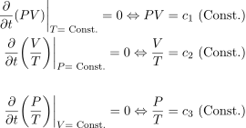
multiplying together,
 .
.
hence  .
.
One can countercheck as follows
 s.t.
s.t.

agrees with

Deduce the kinetic gas equation from conservation of momentum by assumption of elastic collision. Read More
For a cubic container of volume  , the average squared speed
  of one particle of mass in random motion along any -, -,
  -directions is identical

 . For impulse
  during
  , write
  . With particles of rms speed
  , rewrite
  , the pressure being
  , thus the kinetic gas equation,
  .
.
Deduce the magnetic field strength , due to a long straight wire and to a long tightly-packed solenoid both with current carrying, from Biot–Savart law and also from Ampere’s law. Read More
Ampere’s law states that the magnetic flux summed over a closed surface is proportional to the current enclosed by the closed path, i.e.,

By the use of Gaussian pillbox, the magnetic field at a distance from a long straight wire is given by

By the use of amperian loop of length with turns of coils, the coil density being  ,
,


Biot–Savart law of magnetic field states that

At a distance  away from a point
  , let there be a (infinitely) long vertical line
  for
for  . The locus, joining point and any a point on line , is given by
  s.t.
s.t.  and
and  where is the angle of elevation or depression. So,
  ,
,  , and
, and  .
.


Derive Fleming’s left hand rule and right hand rule by vector analysis. Read More


(C004) Observation.
Similarities in formulae for finding the equivalent. Read More
Current in series:

Current in parallel:

Voltage in series:

Voltage in parallel:

Resistance in series:

Resistance in parallel:

Capacitance in series:

Capacitance in parallel:

Inductance in series:

Inductance in parallel:

Similarities in terms of inverse square law. Read More
Newton’s law of gravitational force :

Gravitational field strength:

Coulomb’s law of electrostatic force:

Electric field strength:

Biot–Savart law of magnetic field:
Intensity:

Correspondence between intensive (/intrinsic) and extensive (/extrinsic) properties. Read More
 vs
vs  .
.
 vs
vs 
Comparison between categories. Read More


Perspective from macroscopic to microscopic. Read More

Differences between categories. Read More
Between centre of mass (CM) and centre of gravity (CG):

which depends on mass distribution;

which depends  on gravity variation.
Between mass and weight:
Mass of a body is a constant of matter whereas its weight  is a variable of gravity
  .
.
Between conservative and nonconservative force.
(C005) Formulation.
Ex. 1, Gravity varying with position. Read More
Assumed that the Earth is a perfect sphere of mass , radius , and volume  having uniform mass density
  The weight
  of a test particle at some height above sea level is provided by the Earth’s gravitational force
  with gravitational constant and -dependent gravity
  , i.e.,

For  , please explain the physical meanings of
  ,
,  , and
, and  .
.
Ex. 2, Projectile in parabolic equation. Read More
Let an object be projected from an angle with the level, at an initial speed , and subjected to gravity . Begin with

and

one may write time  in terms of

hence

and thus

Ex. 3, Object and thin lens. Read More
Given for convex (/converging) lens or concave (/diverging) lens
 .
.
When is a constant, write  in terms of

and write  in terms of

s.t. 
For positive and negative focal length  , find for
  ,
,  ,
,  ,
,  ,
,  , and
, and  and hence find whether the image is real or virtual.
(C006) Visualization.
Number line for i. scale, ii. range, and iii. arrow. Read More


Vector Addition by Parallelogram and Head-to-tail Method. Read More

The relationship between displacement graph, velocity graph, and acceleration graph, of independent variable time . Read More

Exercises. (drawing graphs)
The graphs of isobaric process, isochoric/isovolumetric process, isothermal process, and adiabatic process. Read More
1st law of thermodynamic

Isobaric process.

Isochoric/Isovolumetric process.

Isothermal process.

Adiabatic process.

The graphs of average velocity  , instantaneous velocity , average acceleration
  , and instantaneous acceleration .
Field representation by field lines. E.g., electric field, magnetic field, and gravitational field.
Separate  into four parts such that the second part is more than twice the first, the third is twice the fourth, and the fourth is
  more than the first.
J. R. Lux & R. S. Pieters. (1969). Exercises in Elementary Algebra
Roughwork.
Let ,  ,
,  , and
, and  be positive real numbers (
 ) such that
  .
.
Given that

or,

or,

To find the inverse, begin with

proceed with

proceed with

proceed with

proceed with

Hence

and thus

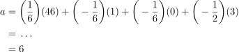


The first number is  , the second
  , the third
  , and the fourth and last
  .
.
When  ,
,  ,
,  ,
,  , and
, and  , give the value of
1. 
2. 
3. 
4. 
5. 
6. 
7. 
8. 
9. 
10. 
11. 
12. 
13. 
14. 
15. 
J. R. Lux & R. S. Pieters. (1969). Exercises in Elementary Algebra
Solution.
1.

2.

3.

4.

5.

6.

7.

8.

9.

10.

11.

12.

13.

14.

15.

Let  ,
,  . Determine whether or not
  .
.
Extracted from M. R. Spiegel. (1969). Schaum’s Outline of Theory and Problems of Real Variables
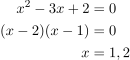
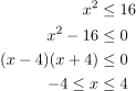
Set and set are described according to property method; if described by the roster method:

Obviously set is a subset of set .
Roughwork.
(set )
(set )
Draw a circle of radius around the center  .
.

As the center of a circle is equidistant from all points on the circumference, using Pythagorean theorem, we have

Attempts. (reinventing the wheel)
Considering the differentials  and
and  , we have

Suppose I do not know the circumference is  long. Let its unknown length be , and let it be partitioned into infinitesimal
  , such that

Assume we may write
 .
.
Expand the right hand side as follows

Then

Suppose I evaluate the integral above by direct substitution by Riemann sum, so the definite integral due to Riemann is given by
 .
.
For  , let
, let  be a regular partition of
 ![[0,2R]](https://physicspupil.com/wp-content/ql-cache/quicklatex.com-fb09bc7b93218a036256f8e15dab160e_l3.svg "Rendered by QuickLaTeX.com") . Then
. Then
 .
.
By right-endpoint approximation for Riemann sums, for each interval ![[x_{i-1},x_i]](https://physicspupil.com/wp-content/ql-cache/quicklatex.com-fad958508b658fc27e7653f8da54b43d_l3.svg "Rendered by QuickLaTeX.com") , we have
, we have
![\displaystyle{x_i=x_0+ix=0+i\bigg[\frac{2R}{n}\bigg]=\frac{2Ri}{n}}](https://physicspupil.com/wp-content/ql-cache/quicklatex.com-4c51443c9a4838ef917c7c064b034ba0_l3.svg "Rendered by QuickLaTeX.com") .
.
Let  . Thus,

Writing the Riemann sum in the form

Inspecting  where
where

I guess, under correction, that  .
.
(to be continued)
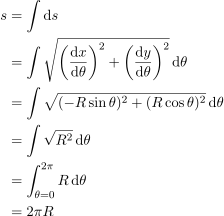
Solution. (arc-length parametrization)
Referring to the equation of locus on the very first line:
 ,
,
then parameterizing  ,
,  by ,
by ,

and computing the derivatives wrt :

Note that

where
 .
.
Then,
(to be continued)
Let  ,
,  , and
, and  . Then,

That is to say, I have made a set of three equations:

in matrix form,

complicating it,

there should be no loss of information; instead, twenty ‘s are gained .

 0 Foreword
This article is sheer homework submitted for earning a grade. And it is not intended to survive academic rigor that it may have any contribution to the current literature.
1 IntroductionMay the author introduce his readers to the history of conceptual change approach.
The term “conceptual change” originated from The Structure of Scientific Revolutions published by Thomas Kuhn in 1962. Kuhn, first a theoretical physicist and later a scholar in the history of science and philosophy, recorded the scientific revolutionary change that took place in physics at that time—from Newtonian mechanics to quantum mechanics. It was nevertheless the tension beneath that surface that loaned its name— the tension between the Received View  and the Theory Reduction
  (Vosniadou, 2007, pp. 1–2). The idea of “conceptual change” and “paradigm shift” transitioned from the philosophy of science into the science education circle equally appropriately, as did the idea of “gestalt switch” and Piaget’s stages of cognitive development from the study of psychology (Lillian Hoddeson, 2007, pp. 26–27).
(The Received View)
"... [t]he attempts by logical positivists and logical empiricists to treat scientific theories as sets of axioms that could be formulated in mathematical logic."
(The Theory Reduction)
"According to theory reduction, a theory that enjoys a high degree of confirmation cannot ever be disconfirmed, but can only be expanded to a theory with a wider scope, or absorbed into a more inclusive and comprehensive theory (see Suppe, 1977)."
Criticisms brought about to ”conceptual change approach” in teaching science are in many aspects, just to list a few:
Hoddeson (2007, pg.27) recalled how his PhD teacher Kuhn studied the “conceptual change” as in “Werner Heisenberg’s intellectual route to his formulation of quantum mechanics”. It can be seen that the term “conceptual change” was originally intended to:
 : make reference to the leap of philosophy of science from the Received View to the Theory Reduction.
 : it is an intrinsic end, an instrumental end, i.e., this approach is descriptive of how science, in particular physics, evolves, but not prescriptive of how science education, inclusive of high school physics, should be attained or designed.
Von Aufschnaiter and Rogge (2010), arguing both theoretically with literature and empirically with their studies on pupils’ conceptual development in physics, posited that pupils are typically lacking in any explanatory conceptual understanding of the content knowledge, and a focus on missing conceptions is much more promising than on misconceptions.
The author couldn’t agree more with all their conclusions, and one of which he cannot overemphasize but ought to restate here is their lately approach—the importance of inclusion of pupils’ misconceptions to teaching is attached to the design of instruction rather than making them an explicit discussion and contrasting them with scientific concepts.
2 Research questionsAndrew A. diSessa (2017, pg. 10) defined “clinical interviewing” to be the technical version of “just talking with people”, and explained how clinical interviewing is connected to instruction. Namely, there are three ways of input.
Input to conjectures and expectations
“Knowing how people think within their zone of felt competence provides important, general and often very specific conjectures about how they can learn from instruction.”
Input to design
“… [S]uch research affects the very goals of instruction (what and when topics should be taught, and how they should be construed), in addition to instructional strategies.”
Input to observation
The clinical interviewer is able to observe “[b]oth the productive and sometimes less productive roles of pre-instructional knowledge”.
To what extent the argument proposed by Von Aufschnaiter and Rogge, namely, that missing conceptions should be focused prior to misconceptions, is confirmed by a clinical interview with a high school physics pupil?
3 MethodologyOne interview was held with a Form 5 pupil, which lasted for eight minutes. A transcript of the interview is in the appendix.
The interviewee had not been taught uniform circular motion before. And the author found it good to have a closed-book talk on this topic with him.
During the interview, there is not any rigid interview protocol, as long as any digression from the subject might still maintain a good understanding between the interviewer and the interviewee.
Notwithstanding that the interview questions should reveal equally likely misconceptions and missing conceptions, the interviewer must have confirmation bias towards a greater likelihood of missing conceptions.
One single interview alone can demonstrate but that at most one interviewee is able to get along with a pre-lesson discussion on expertise and argumentation. And without following up the interviewee’s learning progress, it cannot give evidence to whether such an axiomatic approach as concerns classical physics is a better alternative to the prevailing conceptual change approach.
Findings of interviews with more interviewees and on more diverse and deeper physics topics are in order for presenting themselves to the current literature.
4 Findings and discussionReferring to the transcript from line 25 to 32. The interviewer prompted the interviewee to recall Newton’s first law of motion. The interviewee self-corrected his statement later on though, it might not be an over-extrapolation that he held the impetus theory which is common to physics beginners and laymen.
Such misconception is an instance of ontologically inappropriate miscategorisation of concepts.
Referring to the transcript from line 40 to 65. The interviewee was asked whether or not he could differentiate between speed and velocity. Although the reply being affirmative, it can be inferred that he had not mastered the notion of vectors, and could not tell speed and velocity apart.
When debriefed after the interview, he said that he had never studied vectors in mathematics, as the teaching was not then compulsory. What he could tell was by reciting his bookwork, that speed is the rate of change of distance, and that velocity the rate of change of displacement.
Referring to the transcript from line 68 to 79. It can be extrapolated that a beginner, when first introduced to the centripetal force acting upon an object in circular motion, might be inclined to think there must be some tension between the centre and the orbiter, and dismiss the fact that centripetal force can account for non-contact force, let alone the fact that it is not a force a priori, but a posteriori the net force.
Referring to the transcript from line 97 to 118. It can be observed, that in the scenario when a bus was taking a turn, the interviewee maintained that he should term the force centripetal, despite the fact that its pulling the passenger away from his seat should naturally be termed centrifugal. As an aside, the answer shall depend on which frame—the ground’s or the bus’—is taken reference to, and at this stage it is all too demanding of one high school pupil to tell the difference between inertial and non-inertial frames of reference.
It is worth mentioning, however, that the interviewee admitted that he opted for the term “centripetal” because he had had his supposition that “centrifugal force is a pseudo-force”, based on what disseminated from popular science.
This echoes with that of Ivarsson, Schoultz, and Säljö‘s sociocultural perspective, that human cognition is an interactive process in sociocultural context rather than a purely cognitve one, and “prior knowledge is neither an obstacle nor a prerequisite for conceptual change” (Mayer, 2002, pg. 106).
Referring to the transcript from line 130 to 152. The interviewer asked the interviewee to consider the situation where there is a centripetal force acting on the satellite by the Earth but the satellite will not clash into the Earth. One reading between the lines could identify there might be one assumption held by the interviewee, that “the motion of an object is the same as that of its net force it experiences”.
The interviewee had previously been taught about electrostatics, and he should have rejected the wrong assumption above by giving a counterexample: the path of a charged particle in an E-field is not necessarily the same as the path of field lines.
Referring to the transcript from line 18 to 20. The interviewee was asked whether he could deduce from definition of uniform circular motion that there must exist a net force acting upon it, still less defining it the centripetal force. It was not until in halfway of the interview that he could understand the axiomatic deduction that come up to its existence.
Referring to the transcript from line 147 to 160. The interviewee could not account for the reason that in the presence of a centripetal force an orbiter and the centre are able to keep their distance. The failure might be mostly due to misconception 3, and partly attributed to an over-compartmentalisation of interrelated physics concepts. That is to say, should he relate an orbiter as a projectile with some initial velocity and a downward constant acceleration perpendicular to its motion, he might be given a clue.
5 Conclusions and implications on teachingConceptual change approach has had a long standing reputation for three decades in not only tertiary science teacher education, but teaching high school science also. Care and caution must be taken by educators, to cite Mayer (2002, pg. 127), that it is “… [n]ot a simple process of deletion or replacement of p-prims (i.e., phenomenological primitives), as in contrasting views of conceptual change, but rather a complex process of integration and reorganization”.
The author contends that a pre-instructional talk, chat, or, informal discussion, can help the teacher to design his instruction. Judging misconceptions is with the benefit of hindsight, as searching for missing conceptions is with the benefit of the doubt. Focusing on missing conceptions is indeed more promising than on misconceptions, at least in physics.
Last but not least, as food for thought, if what taught in high school physics is not only classical, but also non-classical (quantum), we have an excuse not to spare the big words—paradigm shift, gestalt switch, conceptual change, and what not. Otherwise, in the senior secondary school physics curriculum, as one in Asian countries, should we not found our education upon normal science, in Kuhn’s terms?
6 ReferencediSessa, A. A. (2017). Knowledge in pieces: an evolving framework for understanding knowing and learning. In Amin, T. G., & Levrini, O. (Eds.). (2017). Converging perspectives on conceptual change: Mapping an emerging paradigm in the learning sciences. Routledge.
Hoddeson, L. (2007). In the wake of Thomas Kuhn’s theory of scientific revolutions: The perspective of an historian of science. In Vosniadou, S., Baltas, A., & Vamvakoussi, X. (Eds.). (2007). Re-framing the conceptual change approach in learning and instruction. Elsevier Ltd.
Mayer, R. E. (2002). Understanding conceptual change: a commentary. In Limón, M. & Mason, L. (Eds.). (2002). Reconsidering conceptual change: issues in theory and practice. Kluwer Academic Publishers
Von Aufschnaiter, C., & Rogge, C. (2010). Misconceptions or missing conceptions?. Eurasia Journal of Mathematics, Science & Technology Education, 6(1).
Vosniadou, S. (2007). The conceptual change approach and its re-framing. In Vosniadou, S., Baltas, A., & Vamvakoussi, X. (Eds.). (2007). Re-framing the conceptual change approach in learning and instruction. Elsevier Ltd.
7 AppendixPlease turn this page over and see Transcript of Interview attached thereafter.
(Submitted on Saturday, 4 May, 2019)