Calculus – Page 3 – Physicspupil

December 13, 2022December 13, 2022

202212131509 Solution to 1985-CE-AMATH-II-6

Find the equations of the two tangents drawn from the point $(-1,0)$ to the parabola $y^2=4x$ .

Roughwork.

$\begin{aligned} y^2 & = 4x \\ 2y\,\mathrm{d}y & = 4\,\mathrm{d}x \\ \frac{\mathrm{d}y}{\mathrm{d}x} & = \frac{2}{y} \\ \end{aligned}$

Let $(a_1,b_1)$ and $(a_2,b_2)$ be two points at which the two tangents touches the parabola. Then,

$\displaystyle{\frac{2}{b_i} =\frac{\mathrm{d}y}{\mathrm{d}x}\bigg|_{(a_i,b_i)} =\frac{b_i-(0)}{a_i-(-1)}}$

By solving two equations in two unknowns:

$\begin{cases} b_i^2 = 2a_i+2 \\ b_i^2 = 4a_i \\ \end{cases} \Longrightarrow\quad \begin{pmatrix} a_i\\b_i \end{pmatrix}_{i=1,2} = \Bigg\{ \begin{pmatrix} 1\\ 2 \end{pmatrix} , \begin{pmatrix} 1 \\ -2 \end{pmatrix} \Bigg\}$

This problem is not to be attempted.

December 13, 2022December 13, 2022

202212131316 Solution to 1983-CE-AMATH-II-3

Use the substitution

$u=1+3x^2$

to evaluate

$\displaystyle{\int_{0}^{1}x^3\sqrt{1+3x^2}\,\mathrm{d}x}$ .

Roughwork.

$\begin{aligned} & \quad\enspace \int_{0}^{1}x^3\sqrt{1+3x^2}\,\mathrm{d}x \\ \dots &\textrm{ let }x=\frac{\tan\theta}{\sqrt{3}}\textrm{ so that }\dots \\ \dots &\textrm{ }\mathrm{d}x=\frac{1}{\sqrt{3}}\sec^2\theta\,\mathrm{d}\theta\textrm{ }\dots \\ \dots &\textrm{ }x=0\Leftrightarrow \theta = 0\textrm{ and }x=1\Leftrightarrow \theta =\frac{\pi}{3}\textrm{ }\dots \\ & = \int_{0}^{\frac{\pi}{3}}\bigg(\frac{\tan\theta}{\sqrt{3}}\bigg)^3\sqrt{1+\tan^2\theta}\,\bigg(\frac{1}{\sqrt{3}}\sec^2\theta\,\mathrm{d}\theta\bigg) \\ & = \frac{1}{9}\int_{0}^{\frac{\pi}{3}}\sec^3\theta\tan^3\theta\,\mathrm{d}\theta \\ \dots & \textrm{ but }\frac{\mathrm{d}(\sec^3\theta )}{\mathrm{d}\theta}=3\sec^2\theta\cdot\sec\theta\tan\theta\textrm{ so }\dots \\ & = \frac{1}{27}\int_{0}^{\frac{\pi}{3}}\tan^2\theta\,\mathrm{d}(\sec^3\theta )\\ \end{aligned}$

Whoops! Read and follow the instructions.

$\begin{aligned} & \quad\enspace \int_{0}^{1}x^3\sqrt{1+3x^2}\,\mathrm{d}x \\ \dots &\textrm{ let }u=1+3x^2\textrm{ then }\mathrm{d}x=\frac{\mathrm{d}u}{6x}\textrm{ }\dots \\ \dots &\textrm{ then }x=0\Leftrightarrow u=1\textrm{ and }x=1\Leftrightarrow u=4\textrm{ }\dots \\ & = \int_{1}^{4}x^3\sqrt{u}\,\bigg(\frac{\mathrm{d}u}{6x}\bigg) \\ & = \frac{1}{6}\int_{1}^{4}\bigg(\frac{u-1}{3}\bigg)\sqrt{u}\,\mathrm{d}u \\ & = \frac{1}{18}\int_{1}^{4}\big( u^{\frac{3}{2}}-u^{\frac{1}{2}}\big)\,\mathrm{d}u \\ & = \frac{1}{18}\bigg[ \frac{2u^{\frac{5}{2}}}{5}-\frac{2u^{\frac{3}{2}}}{3}\bigg]\bigg|_{1}^{4} \\ & = \cdots \\ \end{aligned}$

This problem is not to be attempted.

December 12, 2022December 13, 2022

202212121714 Solution to 1974-CE-AMATH-II-X

A bridge $ABC$ is in the form of the parabola given by the equation

$8y=16-x^2$

as shown in the figure.

The slope of the bridge at the point $P$ is $0.5$ . Find the coordinate of $P$ .

Roughwork.

$\begin{aligned} \bigg|\frac{\mathrm{d}y}{\mathrm{d}x}\bigg| & = \bigg|-\frac{1}{4}x\bigg| \\ 0.5 & = \frac{1}{4}|x| \\ x & = \pm 2 \\ 8y & = 16-(\pm 2)^2 \\ y & = 1.5 \\ \end{aligned}$

Answer. $P(2,1.5)$ .

December 12, 2022December 21, 2022

202212121040 Solution to 1968-CE-AMATH-II-X

Find the maximum and minimum values of $y$ on the curve

$y^2=x(1-x)^2$ .

Sketch the curve.

Roughwork. (true-negative/false-positive example)

All computations in the enclosed section below involving higher-order derivatives than the first are wrong owing to the mistaken assumption

$\times :\quad\displaystyle{\bigg(\frac{\mathrm{d}y}{\mathrm{d}x}\bigg)^2=\frac{(\mathrm{d}y)^2}{(\mathrm{d}x)^2}}$

which was to be detested. Show

$\begin{aligned} y^2 & = x(1-x)^2 \\ & = x(1-2x+x^2) \\ y^2 & = x^3-2x^2+x \\ \end{aligned}$

$\begin{aligned} 2y\,\mathrm{d}y & = 3x^2\,\mathrm{d}x-4x\,\mathrm{d}x+\mathrm{d}x \\ \frac{\mathrm{d}y}{\mathrm{d}x} & = \frac{3x^2-4x+1}{2y} \\ 2(\mathrm{d}y)^2 & = 6x(\mathrm{d}x)^2 - 4(\mathrm{d}x)^2 \\ \bigg(\frac{\mathrm{d}y}{\mathrm{d}x}\bigg)^2 & = 3x-2 \\ \end{aligned}$

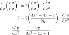
$\begin{aligned} \frac{\mathrm{d}}{\mathrm{d}x}\bigg(\frac{\mathrm{d}y}{\mathrm{d}x}\bigg)^2 & = 2\bigg(\frac{\mathrm{d}y}{\mathrm{d}x}\bigg)\cdot \frac{\mathrm{d}^2y}{\mathrm{d}x^2} \\ 3 & = 2\bigg(\frac{3x^2-4x+1}{2y}\bigg)\cdot \frac{\mathrm{d}^2y}{\mathrm{d}x^2} \\ \frac{\mathrm{d}^2y}{\mathrm{d}x^2} & = \frac{3y}{3x^2-4x+1} \\ \end{aligned}$

$\begin{aligned} y'(x) & = 0 \\ 3x^2-4x+1 & = 0 \\ (3x-1)(x-1) & = 0 \\ x & = \frac{1}{3},1 \\ \end{aligned}$

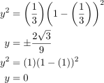
$\begin{aligned} y^2 & = \bigg(\frac{1}{3}\bigg)\bigg(1-\bigg(\frac{1}{3}\bigg)\bigg)^2 \\ y & =\pm\frac{2\sqrt{3}}{9}\\ y^2 & = (1)(1-(1))^2 \\ y & = 0 \\ \end{aligned}$

$\begin{pmatrix}x\\y\end{pmatrix} = \Bigg\{ \begin{pmatrix}\frac{1}{3}\\ -\frac{2\sqrt{3}}{9} \end{pmatrix}, \begin{pmatrix}\frac{1}{3}\\ \frac{2\sqrt{3}}{9} \end{pmatrix}, \begin{pmatrix}1\\0\end{pmatrix}\Bigg\}$ are extrema.

$\begin{aligned} y''(x) & = 0 \\ 3y & = 0 \\ \pm\sqrt{x(1-x)^2} & = 0 \\ x(1-x)^2 & = 0 \\ x & = 0,1 \\ \end{aligned}$

$\begin{pmatrix}x\\y\end{pmatrix} = \bigg\{ \begin{pmatrix}0\\ 0 \end{pmatrix}, \begin{pmatrix}1\\ 0\end{pmatrix}\bigg\}$ are inflexions.

To answer whether

$\displaystyle{\frac{\mathrm{d}^2y}{\mathrm{d}x^2}}\bigg|_{\big( \frac{1}{3},\pm\frac{2\sqrt{3}}{9}\big)}$

is positive or negative is critical to yielding the maximum and the minimum values of the function.

The correction is left a $\textrm{\scriptsize{MUST}}$ for the author.

December 12, 2022December 12, 2022

202212121004 Solution to 1968-CE-AMATH-II-X

Find $\displaystyle{\frac{\mathrm{d}y}{\mathrm{d}x}}$ if

$ax^2+2hxy+by^2+2gx+2fy+c=0$ .

Roughwork.

$\begin{aligned} ax^2+2hxy+by^2+2gx+2fy+c & =0 \\ 2ax\,\mathrm{d}x+2h(x\,\mathrm{d}y+y\,\mathrm{d}x)+2by\,\mathrm{d}y+2g\,\mathrm{d}x+2f\,\mathrm{d}y & = 0 \\ 2ax + 2h\bigg( x\frac{\mathrm{d}y}{\mathrm{d}x}+y\bigg) +2by\frac{\mathrm{d}y}{\mathrm{d}x}+2g+2f\frac{\mathrm{d}y}{\mathrm{d}x} & = 0 \\ (ax+hy+g) + (hx+by+f)\frac{\mathrm{d}y}{\mathrm{d}x} & = 0 \\ -\frac{ax+hy+g}{hx+by+f} & = y' \\ \end{aligned}$

This problem is not to be attempted.

December 12, 2022December 12, 2022

202212120958 Solution to 1967-CE-AMATH-II-X

A spherical balloon is of diameter $x$ . By what approximate amount does the volume increases, if the diameter is increased by a very small amount $\Delta x$ ?

Roughwork.

$\begin{aligned} V & = \frac{4}{3}\pi x^3 \\ \Delta V & = 4\pi x^2\,\Delta x \\ \end{aligned}$

September 28, 2022October 24, 2022

202209281050 Exercise 22.2 (Q23)

An electric field is given by $\overrightarrow{E}=E_0\,\hat{\jmath}$ , where $E_0$ is a constant. Find the potential as a function of position, taking $V=0$ at $y=0$ .

_{Extracted from R. Wolfson. (2016). Essential University Physics.}

Background.

Electric field vector $\overrightarrow{E}$ is related to electric potential $V$ by:

$\displaystyle{\overrightarrow{E}= -\bigg( \frac{\partial V}{\partial x}\,\hat{\mathbf{i}} + \frac{\partial V}{\partial y}\,\hat{\mathbf{j}} + \frac{\partial V}{\partial z}\,\hat{\mathbf{k}} \bigg)}$

or reversely,

$\displaystyle{V(r)=-\int\overrightarrow{E}\cdot\mathrm{d}\vec{r}}$ .

Write

$\displaystyle{(0,E_0,0) = \bigg( -\frac{\partial V}{\partial x},-\frac{\partial V}{\partial y},-\frac{\partial V}{\partial z}\bigg) }$

that implies $V=V(y)$ is $x$ – and $z$ -independent.

Hence

$\begin{aligned} V(y) & = -\int E_0\,\mathrm{d}y \\ & = -E_0y+C\qquad \textrm{for some constant }C \\ \because\enspace 0 & = V(y=0) = -E_0(0)+C \\ \Rightarrow C& = 0 \\ \therefore\enspace V&=V(y)=-E_0y\\ \end{aligned}$

June 8, 2022October 24, 2022

202206081501 Exercise 4.1 (Q15)

In an electric circuit with a supplied voltage (emf) $E$ , a resistor with resistance $r_0$ , and an inductor with reactance $x_0$ , suppose you want to add a second resistor. If $r$ represents the resistance of this second resistor then the power $P$ delivered to that resistor is given by

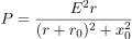
$\displaystyle{P=\frac{E^2r}{(r+r_0)^2+x_0^2}}$

with $E$ , $r_0$ , and $x_0$ treated as constants. For which value of $r$ is the power $P$ maximized?

_{extracted from Michael Corral. (2020). Elementary Calculus}

Lemma. (quotient rule)

Let $f(x)=\displaystyle{\frac{g(x)}{h(x)}}$ , where both $g$ and $h$ are differentiable and $h(x)\neq 0$ . The quotient rule states that the derivative of $f(x)$ is

$f'(x)=\displaystyle{\frac{g'(x)h(x)-g(x)h'(x)}{h(x)^2}}$

_{Wikipedia on Quotient Rule}

Roughwork.

Defining

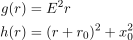
$\begin{aligned} g(r) & = E^2r\\ h(r) & = (r+r_0)^2+x_0^2\\ \end{aligned}$

and

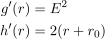
$\begin{aligned} g'(r) & = E^2\\ h'(r) & = 2(r+r_0)\\ \end{aligned}$

then

$\displaystyle{\frac{\mathrm{d}P}{\mathrm{d}r}}=0\Longrightarrow g'(r)h(r)-g(r)h'(r)=0$

Computing as follows

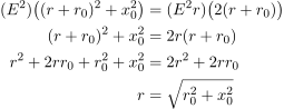
$\begin{aligned} (E^2)\big( (r+r_0)^2+x_0^2 \big) & = (E^2r)\big( 2(r+r_0) \big) \\ (r+r_0)^2+x_0^2 & = 2r(r+r_0) \\ r^2+2rr_0+r_0^2 +x_0^2 & = 2r^2+2rr_0 \\ r & = \sqrt{r_0^2+x_0^2} \\ \end{aligned}$

The mathematically formal way is to show that

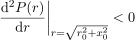
$\displaystyle{\frac{\mathrm{d}^2P(r)}{\mathrm{d}r}\bigg|_{r=\sqrt{r^2_0+x_0^2}}}<0$

But from a physical point of view, assume that the electric currents $i$ passing through every components in series are the same, and the potential difference across each total up to the supplied voltage, namely,

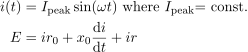
$\begin{aligned} i(t) & = I_{\textrm{peak}}\sin (\omega t) \textrm{ where }I_{\textrm{peak}}\textrm{= const.} \\ E & = ir_0+x_0\frac{\mathrm{d}i}{\mathrm{d}t}+ir \\ \end{aligned}$

The power $P$ delivered to resistor $r$ is given by the formula

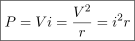
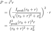
$\boxed{P=Vi=\displaystyle{\frac{V^2}{r}}=i^2r}$

and the only way to maximize $P$ , is to maximize either or both $i$ and $V$ .

Solving for a first-order ordinary differential equation:

$f(r,i,i')= ir_0+x_0i'+ir-E=0$

deriving current $i$ wrt $\omega t$ , we have

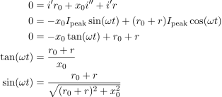
$\begin{aligned} 0 & = i'r_0+x_0i''+i'r \\ 0 & = -x_0I_{\textrm{peak}}\sin (\omega t)+(r_0+r)I_{\textrm{peak}}\cos (\omega t) \\ 0 & = -x_0\tan (\omega t) + r_0+r \\ \tan (\omega t) & = \frac{r_0+r}{x_0} \\ \sin (\omega t)&=\frac{r_0+r}{\sqrt{(r_0+r)^2+x_0^2}} \\ \end{aligned}$

Thus $i(r)=\displaystyle{I_{\textrm{peak}}\frac{r_0+r}{\sqrt{(r_0+r)^2+x_0^2}}}$

$\begin{aligned} P & = i^2r \\ & = \bigg(\frac{I_{\textrm{peak}}(r_0+r)}{\sqrt{(r_0+r)^2+x_0^2}}\bigg)^2 \cdot r \\ & = \frac{I_{\textrm{peak}}^2(r_0+r)^2r}{(r_0+r)^2+x_0^2} \\ \end{aligned}$

(to be continued)

Recall the relation between root mean square (rms) values and peak values:

$\begin{aligned} V_{\textrm{rms}} & = \frac{V_\textrm{peak}}{\sqrt{2}} \\ I_{\textrm{rms}} & = \frac{I_\textrm{peak}}{\sqrt{2}} \\ \end{aligned}$

Recall also that the resistance $R_L$ of an ideal inductor is zero ( $=0$ ), and that after the circuit has shortly reached steady state (i.e., constant current $i$ anywhere/anytime), the potential difference ( $\textrm{p.d.}$ ) or voltage drop ( $\Delta V$ ) across the inductor will become zero ( $=0$ ) before long.

Try again,

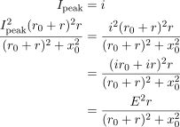
$\begin{aligned} I_{\textrm{peak}} & = i \\ \frac{I_{\textrm{peak}}^2(r_0+r)^2r}{(r_0+r)^2+x_0^2} & = \frac{i^2(r_0+r)^2r}{(r_0+r)^2+x_0^2} \\ & = \frac{(ir_0+ir)^2r}{(r_0+r)^2+x_0^2} \\ & = \frac{E^2r}{(r_0+r)^2+x_0^2} \\ \end{aligned}$

The derivative test seems inevitable. Maybe you could show that resistance $r=\sqrt{r_0^2+x_0^2}$ maximizes power $P$ , simply by drawing a phasor diagram?

(to be continued)

June 8, 2022October 24, 2022

202206081349 Exercise 4.1 (Q12)

The phase velocity $v$ of a capillary wave with surface tension $T$ and water density $p$ is

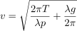
$\displaystyle{v=\sqrt{\frac{2\pi T}{\lambda p}+\frac{\lambda g}{2\pi}}}$

where $\lambda$ is the wavelength. Find the value of $\lambda$ that minimizes $v$ .

_{extracted from Michael Corral. (2020). Elementary Calculus.}

Setup.

Let $v=v(u(\lambda ))$ s.t.

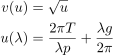
$\begin{aligned} v(u) &=\sqrt{u} \\ u(\lambda ) & =\frac{2\pi T}{\lambda p}+\frac{\lambda g}{2\pi } \\ \end{aligned}$

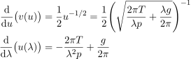
$\begin{aligned} \frac{\mathrm{d}}{\mathrm{d}u}\big( v(u)\big) & = \frac{1}{2}u^{-1/2}=\frac{1}{2}\Bigg(\sqrt{\frac{2\pi T}{\lambda p}+\frac{\lambda g}{2\pi}}\Bigg)^{-1} \\ \frac{\mathrm{d}}{\mathrm{d}\lambda}\big( u(\lambda )\big) & = -\frac{2\pi T}{\lambda^2p}+\frac{g}{2\pi} \\ \end{aligned}$

Hence,

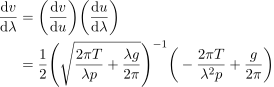
$\begin{aligned} \frac{\mathrm{d}v}{\mathrm{d}\lambda} & = \bigg(\frac{\mathrm{d}v}{\mathrm{d}u}\bigg) \bigg(\frac{\mathrm{d}u}{\mathrm{d}\lambda}\bigg) \\ & = \frac{1}{2}\Bigg(\sqrt{\frac{2\pi T}{\lambda p}+\frac{\lambda g}{2\pi}}\Bigg)^{-1}\bigg(-\frac{2\pi T}{\lambda^2p}+\frac{g}{2\pi}\bigg) \\ \end{aligned}$

Working.

For $\displaystyle{\frac{\mathrm{d}v}{\mathrm{d}\lambda}}=0$ requires:

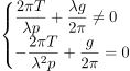
$\begin{cases} \displaystyle{\frac{2\pi T}{\lambda p}+\frac{\lambda g}{2\pi}} \neq 0 \\ \displaystyle{-\frac{2\pi T}{\lambda^2p}+\frac{g}{2\pi}}= 0 \\ \end{cases}$

Answer.

We have the satisfying stationary point:

$\lambda_0 =\displaystyle{2\pi\sqrt{\frac{T}{pg}}}$ .

It remains to be verified that this is a global minimum indeed.

(to be continued)

June 1, 2022October 24, 2022

202206011159 Problem 5E (Q25)

Test each of the following differentials to see whether they are exact, using two methods for each:

(a) $-y\sin x\,\mathrm{d}x+\cos x\,\mathrm{d}y$ ,

(b) $y\,\mathrm{d}x+x\,\mathrm{d}y$ ,
(c) $yx^3e^x\,\mathrm{d}x+x^3e^x\,\mathrm{d}y$ ,
(d) $(1+x)ye^x\,\mathrm{d}x+xe^x\,\mathrm{d}y$ ,
(e) $4x^3y^{-2}\,\mathrm{d}x-2x^4y^{-3}\,\mathrm{d}y$ .

_{K. S. Stowe. (2007). An Introduction to Thermodynamics and Statistical Mechanics}

Revision. (exact differentials)

The differential of a function is given by Eq. (5.8):

$\mathrm{d}F=\displaystyle{\frac{\partial F}{\partial x}\,\mathrm{d}x+\frac{\partial F}{\partial y}\,\mathrm{d}y}$ .

Therefore, one way to determine whether a differential given by Eq. (5.9):

$\mathrm{d}\Phi =g(x,y)\,\mathrm{d}x+h(x,y)\,\mathrm{d}y$

is exact is to see whether we can find some function $F(x,y)$ such that

$\displaystyle{\frac{\partial F}{\partial x}=g(x,y)}\qquad \textrm{and}\qquad\displaystyle{\frac{\partial F}{\partial y}=h(x,y)}$ .

If we can, the differential is exact, and if we can’t, it is inexact. Alternatively, we can use the identity

$\displaystyle{\frac{\partial^2F}{\partial y\partial x}=\frac{\partial^2F}{\partial x\partial y}}$ .

Combining this with equations (5.8) and (5.9), we can see that for exact differentials, Eq. (5.10):

$\displaystyle{\frac{\partial g}{\partial y}=\frac{\partial h}{\partial x}}$ .

_{Text on pg. 89, Sec. E, Ch. 5}

Roughwork.

(a)

We can see that this is indeed an exact differential of the function

$F=y\cos x+\textrm{constant}$ ,

because

$\displaystyle{\frac{\partial F}{\partial x}=-y\sin x}\qquad\textrm{and}\qquad\displaystyle{\frac{\partial F}{\partial y}=\cos x}$ .

Or we can use Eq. (5.10). For this example $g=-y\sin x$ and $h=\cos x$ , so

$\displaystyle{\frac{\partial g}{\partial y}=-\sin x}\qquad\textrm{and}\qquad\displaystyle{\frac{\partial h}{\partial x}=-\sin x}$ .

The two are the same, so the differential is exact.

Parts (b) to (e) are left to the reader as an exercise. Cf. analytic functions et Cauchy-Riemann equations.