Physicspupil – Page 22

July 7, 2022October 24, 2022

202207071143 Exercise 18.1 (Q1)

The Sun is a yellow star and emits most of its radiation in the yellow portion of the spectrum. If the sun’s radiation peaks at a frequency of $5.20\times 10^{14}\,\mathrm{Hz}$ , how much energy is emitted by one photon of this visible yellow light?

_{J. B., Hickman. (2002). Problem-Solving Exercises in Physics}

Roughwork.

In joules,

$\begin{aligned} E&=hf \\ & = (6.63\times 10^{-34}\,\mathrm{J\cdot s})(5.20\times 10^{14}\,\mathrm{Hz}) \\ & = 3.4476\times 10^{-19}\,\mathrm{J} \\ \end{aligned}$

In electron volts,

$\begin{aligned} E & = \frac{3.4476\times 10^{-19}\,\mathrm{J}}{1.60\times 10^{-19}\,\mathrm{J/eV}} \\ & = 2.15475\,\mathrm{eV} \\ \end{aligned}$

July 6, 2022October 24, 2022

202207061152 Solution to 1971-CE-AMATH-I-XX

If $k$ is an integer, simplify

$\displaystyle{\cos\bigg[ \frac{1}{2}(4k+1)\pi +\theta \bigg]\tan\bigg[\frac{1}{2}(4k+3)\pi -\theta \bigg]}$ .

Roughwork.

First,

$\begin{aligned} & \quad \cos\bigg[ \frac{1}{2}(4k+1)\pi +\theta \bigg]\tan\bigg[\frac{1}{2}(4k+3)\pi -\theta \bigg] \\ & = \cos\bigg( 2k\pi+\frac{\pi}{2}+\theta \bigg) \tan \bigg( 2k\pi+\frac{3\pi}{2}-\theta \bigg) \\ \dots\textrm{as } &\textrm{are}\cos (\angle ),\tan (\angle )\textrm{ shifted by full periods, \textit{i.e.}, }k\cdot 2\pi\,\dots \\ & = \cos\bigg(\frac{\pi}{2}+\theta\bigg) \tan \bigg(\frac{3\pi}{2}-\theta \bigg) \\ \end{aligned}$

Second,

recall that

$\begin{aligned} \textrm{(in radians)} & \quad\textrm{(in degrees)} \\ \pi & = 180^\circ \\ \frac{\pi}{2} & = 90^\circ \\ \frac{3\pi}{2} & = 270^\circ\textrm{ \scriptsize{OR} }-90^\circ = -\frac{\pi}{2}\\ \end{aligned}$

Hence,

$\begin{aligned} & \quad \cos\bigg(\frac{\pi}{2}+\theta\bigg) \tan \bigg(\frac{3\pi}{2}-\theta \bigg) \\ & = \cos\bigg(\frac{\pi}{2}+\theta\bigg) \tan \bigg(-\frac{\pi}{2}-\theta \bigg) \\ & = \cos\bigg(\frac{\pi}{2}+\theta\bigg) \tan \bigg[ -\bigg(\frac{\pi}{2}+\theta \bigg)\bigg] \\ \dots &\textrm{ as }\tan(-\theta )=-\tan\theta \enspace\dots \\ & = -\cos\bigg(\frac{\pi}{2}+\theta\bigg) \tan \bigg(\frac{\pi}{2}+\theta\bigg) \\ \end{aligned}$ .

Recall that

$\begin{aligned} \because \enspace & \tan\theta = \frac{\sin\theta}{\cos\theta} \\ \therefore \enspace & \cos\theta\tan\theta = \sin\theta \\ \end{aligned}$ .

Hence,

$\begin{aligned} &\quad -\cos\bigg( \frac{\pi}{2}+\theta\bigg)\tan\bigg( \frac{\pi}{2}+\theta\bigg) \\ & = -\sin\bigg( \frac{\pi}{2}+\theta\bigg) \\ \end{aligned}$

Third,

recall that

$\displaystyle{\sin \bigg(\theta\pm\frac{\pi}{2}\bigg)}=\pm\cos\theta$ .

$\begin{aligned} &\quad -\sin \bigg( \frac{\pi}{2}+\theta\bigg) \\ & = -\cos\theta \\ \end{aligned}$

Answer.

$\displaystyle{\cos\bigg[ \frac{1}{2}(4k+1)\pi +\theta \bigg]\tan\bigg[\frac{1}{2}(4k+3)\pi -\theta \bigg]}=-\cos\theta$ .

July 5, 2022October 24, 2022

202207051339 Solution to 1974-CE-AMATH-I-XX

(a) In the figure below, $ABCDEF$ is a regular hexagon. Which one of the $6$ vectors $\overrightarrow{AD}$ , $\overrightarrow{DA}$ , $\overrightarrow{FC}$ , $\overrightarrow{CF}$ , $\overrightarrow{EB}$ , $\overrightarrow{BE}$ is equal to $\overrightarrow{AB}+\overrightarrow{BC}+\overrightarrow{DC}$ ?

(b) $\mathbf{u}$ and $\mathbf{v}$ are unit vectors making an angle $60^\circ$ with each other as shown in the figure below. $AB$ is a vector making an angle $30^\circ$ with $\mathbf{u}$ and $|\overrightarrow{AB}|=2$ . Express $\overrightarrow{AB}$ in terms of $\mathbf{u}$ and $\mathbf{v}$ .

(c) In the figure below, $\angle B=90^\circ$ and $m(\overrightarrow{AB})=10$ . Calculate $\overrightarrow{AB}\cdot\overrightarrow{AC}$ .

(a)

$\begin{aligned} \mathbf{AD} & = -\mathbf{DA} \\ |\mathbf{AD}| & = |\mathbf{DA}| \\ \mathbf{FC} & = -\mathbf{CF} \\ |\mathbf{FC}| & = |\mathbf{CF}| \\ \mathbf{EB} & = -\mathbf{BE} \\ |\mathbf{EB}| & = |\mathbf{BE}| \\ \end{aligned}$

Ans. $\mathbf{FC}$ $\textrm{\scriptsize{OR}}$ $\overrightarrow{FC}$ by inspection.

Working.

$\begin{aligned} &\quad \mathbf{AB} + \mathbf{BC} + \mathbf{DC} \\ & = (\mathbf{AB} + \mathbf{BC}) + \mathbf{DC} \\ & = \mathbf{AC} + \mathbf{DC} \\ \dots & \textrm{ as }\mathbf{AC}=\mathbf{FD} \enspace\dots \\ & = \mathbf{FD} + \mathbf{DC} \\ & = \mathbf{FC} \\ \end{aligned}$

(b)

Write, in Cartesian components of unit vectors $\hat{\mathbf{i}}$ and $\hat{\mathbf{j}}$ , the following:

$\begin{aligned} \mathbf{AB} & = |\mathbf{AB}|\cos 30^\circ\,\hat{\mathbf{i}} + |\mathbf{AB}|\sin 30^\circ\,\hat{\mathbf{j}} \\ & = 2\cos 30^\circ\,\hat{\mathbf{i}} + 2\sin 30^\circ\,\hat{\mathbf{j}} \\ & = \sqrt{3}\,\hat{\mathbf{i}} + 1\,\hat{\mathbf{j}} \\ \end{aligned}$

and similarly,

$\begin{aligned} \mathbf{u} & = |\mathbf{u}|\,\hat{\mathbf{i}} \\ \mathbf{v} & = |\mathbf{v}|\cos 60^\circ\,\hat{\mathbf{i}} + |\mathbf{v}|\sin 60^\circ\,\hat{\mathbf{j}}\\ & \\ \because\enspace & \mathbf{u}, \mathbf{v}\textrm{ are unit vectors} \\ \therefore\enspace & |\mathbf{u}|=|\mathbf{v}|=1 \\ & \\ \mathbf{u} & = \hat{\mathbf{i}} \\ \mathbf{v} & = \frac{1}{2}\,\hat{\mathbf{i}} + \frac{\sqrt{3}}{2} \hat{\mathbf{j}} \\ \end{aligned}$

$\begin{aligned} \begin{bmatrix} \mathbf{u} \\ \mathbf{v} \end{bmatrix} & = \begin{bmatrix} 1 & 0 \\ \frac{1}{2} & \frac{\sqrt{3}}{2} \end{bmatrix} \begin{bmatrix} \hat{\mathbf{i}} \\ \hat{\mathbf{j}} \end{bmatrix} \\ \begin{bmatrix} \hat{\mathbf{i}} \\ \hat{\mathbf{j}} \end{bmatrix} & = \begin{bmatrix} 1 & 0 \\ \frac{1}{2} & \frac{\sqrt{3}}{2} \end{bmatrix}^{-1}\begin{bmatrix} \mathbf{u} \\ \mathbf{v} \end{bmatrix} \\ \end{aligned}$

Lemma. (Inversion of 2-by-2 matrices)

For $2\times 2$ matrices, inversion can be done as follows:

$\begin{aligned} \mathbf{A}^{-1} & = \begin{bmatrix} a & b \\ c & d \end{bmatrix}^{-1} \\ & = \frac{1}{\mathrm{det}\mathbf{A}}\begin{bmatrix} d & -b \\ -c & a \end{bmatrix} \\ & = \frac{1}{ad-bc}\begin{bmatrix} d & -b \\ -c & a \end{bmatrix} \\ \end{aligned}$

_{Wikipedia on Invertible matrix}

Then,

$\begin{bmatrix} 1 & 0 \\ \frac{1}{2} & \frac{\sqrt{3}}{2}\end{bmatrix}^{-1} = \begin{bmatrix} 1 & 0 \\ -\frac{1}{\sqrt{3}} & \frac{2}{\sqrt{3}} \end{bmatrix}$

so that

$\begin{bmatrix} \hat{\mathbf{i}} \\ \hat{\mathbf{j}} \end{bmatrix} = \begin{bmatrix} 1 & 0 \\ -\frac{1}{\sqrt{3}} & \frac{2}{\sqrt{3}} \end{bmatrix}\begin{bmatrix}\mathbf{u} \\ \mathbf{v}\end{bmatrix}$

Thus

$\begin{aligned} \mathbf{AB} & =\begin{pmatrix} \sqrt{3} & 1\end{pmatrix}\begin{bmatrix}\hat{\mathbf{i}} \\ \hat{\mathbf{j}} \end{bmatrix} \\ & = \begin{pmatrix} \sqrt{3} & 1\end{pmatrix} \begin{bmatrix} 1 & 0 \\ -\frac{1}{\sqrt{3}} & \frac{2}{\sqrt{3}} \end{bmatrix} \begin{bmatrix}\mathbf{u} \\ \mathbf{v}\end{bmatrix} \\ & = \begin{bmatrix} \frac{2}{\sqrt{3}} & \frac{2}{\sqrt{3}} \end{bmatrix}\begin{bmatrix}\mathbf{u} \\ \mathbf{v}\end{bmatrix} \\ &=\frac{2}{\sqrt{3}}\,\mathbf{u}+\frac{2}{\sqrt{3}}\,\mathbf{v} \\ \end{aligned}$

There might be some mistake if conceptually.

(c)

I don’t know how. Skip it.

June 8, 2022October 24, 2022

202206081501 Exercise 4.1 (Q15)

In an electric circuit with a supplied voltage (emf) $E$ , a resistor with resistance $r_0$ , and an inductor with reactance $x_0$ , suppose you want to add a second resistor. If $r$ represents the resistance of this second resistor then the power $P$ delivered to that resistor is given by

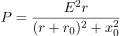
$\displaystyle{P=\frac{E^2r}{(r+r_0)^2+x_0^2}}$

with $E$ , $r_0$ , and $x_0$ treated as constants. For which value of $r$ is the power $P$ maximized?

_{extracted from Michael Corral. (2020). Elementary Calculus}

Lemma. (quotient rule)

Let $f(x)=\displaystyle{\frac{g(x)}{h(x)}}$ , where both $g$ and $h$ are differentiable and $h(x)\neq 0$ . The quotient rule states that the derivative of $f(x)$ is

$f'(x)=\displaystyle{\frac{g'(x)h(x)-g(x)h'(x)}{h(x)^2}}$

_{Wikipedia on Quotient Rule}

Roughwork.

Defining

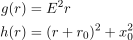
$\begin{aligned} g(r) & = E^2r\\ h(r) & = (r+r_0)^2+x_0^2\\ \end{aligned}$

and

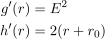
$\begin{aligned} g'(r) & = E^2\\ h'(r) & = 2(r+r_0)\\ \end{aligned}$

then

$\displaystyle{\frac{\mathrm{d}P}{\mathrm{d}r}}=0\Longrightarrow g'(r)h(r)-g(r)h'(r)=0$

Computing as follows

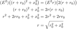
$\begin{aligned} (E^2)\big( (r+r_0)^2+x_0^2 \big) & = (E^2r)\big( 2(r+r_0) \big) \\ (r+r_0)^2+x_0^2 & = 2r(r+r_0) \\ r^2+2rr_0+r_0^2 +x_0^2 & = 2r^2+2rr_0 \\ r & = \sqrt{r_0^2+x_0^2} \\ \end{aligned}$

The mathematically formal way is to show that

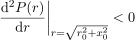
$\displaystyle{\frac{\mathrm{d}^2P(r)}{\mathrm{d}r}\bigg|_{r=\sqrt{r^2_0+x_0^2}}}<0$

But from a physical point of view, assume that the electric currents $i$ passing through every components in series are the same, and the potential difference across each total up to the supplied voltage, namely,

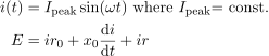
$\begin{aligned} i(t) & = I_{\textrm{peak}}\sin (\omega t) \textrm{ where }I_{\textrm{peak}}\textrm{= const.} \\ E & = ir_0+x_0\frac{\mathrm{d}i}{\mathrm{d}t}+ir \\ \end{aligned}$

The power $P$ delivered to resistor $r$ is given by the formula

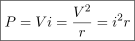
$\boxed{P=Vi=\displaystyle{\frac{V^2}{r}}=i^2r}$

and the only way to maximize $P$ , is to maximize either or both $i$ and $V$ .

Solving for a first-order ordinary differential equation:

$f(r,i,i')= ir_0+x_0i'+ir-E=0$

deriving current $i$ wrt $\omega t$ , we have

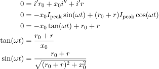
$\begin{aligned} 0 & = i'r_0+x_0i''+i'r \\ 0 & = -x_0I_{\textrm{peak}}\sin (\omega t)+(r_0+r)I_{\textrm{peak}}\cos (\omega t) \\ 0 & = -x_0\tan (\omega t) + r_0+r \\ \tan (\omega t) & = \frac{r_0+r}{x_0} \\ \sin (\omega t)&=\frac{r_0+r}{\sqrt{(r_0+r)^2+x_0^2}} \\ \end{aligned}$

Thus $i(r)=\displaystyle{I_{\textrm{peak}}\frac{r_0+r}{\sqrt{(r_0+r)^2+x_0^2}}}$

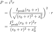
$\begin{aligned} P & = i^2r \\ & = \bigg(\frac{I_{\textrm{peak}}(r_0+r)}{\sqrt{(r_0+r)^2+x_0^2}}\bigg)^2 \cdot r \\ & = \frac{I_{\textrm{peak}}^2(r_0+r)^2r}{(r_0+r)^2+x_0^2} \\ \end{aligned}$

(to be continued)

Recall the relation between root mean square (rms) values and peak values:

$\begin{aligned} V_{\textrm{rms}} & = \frac{V_\textrm{peak}}{\sqrt{2}} \\ I_{\textrm{rms}} & = \frac{I_\textrm{peak}}{\sqrt{2}} \\ \end{aligned}$

Recall also that the resistance $R_L$ of an ideal inductor is zero ( $=0$ ), and that after the circuit has shortly reached steady state (i.e., constant current $i$ anywhere/anytime), the potential difference ( $\textrm{p.d.}$ ) or voltage drop ( $\Delta V$ ) across the inductor will become zero ( $=0$ ) before long.

Try again,

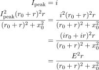
$\begin{aligned} I_{\textrm{peak}} & = i \\ \frac{I_{\textrm{peak}}^2(r_0+r)^2r}{(r_0+r)^2+x_0^2} & = \frac{i^2(r_0+r)^2r}{(r_0+r)^2+x_0^2} \\ & = \frac{(ir_0+ir)^2r}{(r_0+r)^2+x_0^2} \\ & = \frac{E^2r}{(r_0+r)^2+x_0^2} \\ \end{aligned}$

The derivative test seems inevitable. Maybe you could show that resistance $r=\sqrt{r_0^2+x_0^2}$ maximizes power $P$ , simply by drawing a phasor diagram?

(to be continued)

June 8, 2022October 24, 2022

202206081349 Exercise 4.1 (Q12)

The phase velocity $v$ of a capillary wave with surface tension $T$ and water density $p$ is

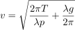
$\displaystyle{v=\sqrt{\frac{2\pi T}{\lambda p}+\frac{\lambda g}{2\pi}}}$

where $\lambda$ is the wavelength. Find the value of $\lambda$ that minimizes $v$ .

_{extracted from Michael Corral. (2020). Elementary Calculus.}

Setup.

Let $v=v(u(\lambda ))$ s.t.

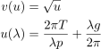
$\begin{aligned} v(u) &=\sqrt{u} \\ u(\lambda ) & =\frac{2\pi T}{\lambda p}+\frac{\lambda g}{2\pi } \\ \end{aligned}$

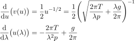
$\begin{aligned} \frac{\mathrm{d}}{\mathrm{d}u}\big( v(u)\big) & = \frac{1}{2}u^{-1/2}=\frac{1}{2}\Bigg(\sqrt{\frac{2\pi T}{\lambda p}+\frac{\lambda g}{2\pi}}\Bigg)^{-1} \\ \frac{\mathrm{d}}{\mathrm{d}\lambda}\big( u(\lambda )\big) & = -\frac{2\pi T}{\lambda^2p}+\frac{g}{2\pi} \\ \end{aligned}$

Hence,

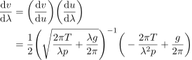
$\begin{aligned} \frac{\mathrm{d}v}{\mathrm{d}\lambda} & = \bigg(\frac{\mathrm{d}v}{\mathrm{d}u}\bigg) \bigg(\frac{\mathrm{d}u}{\mathrm{d}\lambda}\bigg) \\ & = \frac{1}{2}\Bigg(\sqrt{\frac{2\pi T}{\lambda p}+\frac{\lambda g}{2\pi}}\Bigg)^{-1}\bigg(-\frac{2\pi T}{\lambda^2p}+\frac{g}{2\pi}\bigg) \\ \end{aligned}$

Working.

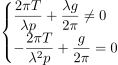
For $\displaystyle{\frac{\mathrm{d}v}{\mathrm{d}\lambda}}=0$ requires:

$\begin{cases} \displaystyle{\frac{2\pi T}{\lambda p}+\frac{\lambda g}{2\pi}} \neq 0 \\ \displaystyle{-\frac{2\pi T}{\lambda^2p}+\frac{g}{2\pi}}= 0 \\ \end{cases}$

Answer.

We have the satisfying stationary point:

$\lambda_0 =\displaystyle{2\pi\sqrt{\frac{T}{pg}}}$ .

It remains to be verified that this is a global minimum indeed.

(to be continued)

June 1, 2022October 24, 2022

202206011159 Problem 5E (Q25)

Test each of the following differentials to see whether they are exact, using two methods for each:

(a) $-y\sin x\,\mathrm{d}x+\cos x\,\mathrm{d}y$ ,

(b) $y\,\mathrm{d}x+x\,\mathrm{d}y$ ,
(c) $yx^3e^x\,\mathrm{d}x+x^3e^x\,\mathrm{d}y$ ,
(d) $(1+x)ye^x\,\mathrm{d}x+xe^x\,\mathrm{d}y$ ,
(e) $4x^3y^{-2}\,\mathrm{d}x-2x^4y^{-3}\,\mathrm{d}y$ .

_{K. S. Stowe. (2007). An Introduction to Thermodynamics and Statistical Mechanics}

Revision. (exact differentials)

The differential of a function is given by Eq. (5.8):

$\mathrm{d}F=\displaystyle{\frac{\partial F}{\partial x}\,\mathrm{d}x+\frac{\partial F}{\partial y}\,\mathrm{d}y}$ .

Therefore, one way to determine whether a differential given by Eq. (5.9):

$\mathrm{d}\Phi =g(x,y)\,\mathrm{d}x+h(x,y)\,\mathrm{d}y$

is exact is to see whether we can find some function $F(x,y)$ such that

$\displaystyle{\frac{\partial F}{\partial x}=g(x,y)}\qquad \textrm{and}\qquad\displaystyle{\frac{\partial F}{\partial y}=h(x,y)}$ .

If we can, the differential is exact, and if we can’t, it is inexact. Alternatively, we can use the identity

$\displaystyle{\frac{\partial^2F}{\partial y\partial x}=\frac{\partial^2F}{\partial x\partial y}}$ .

Combining this with equations (5.8) and (5.9), we can see that for exact differentials, Eq. (5.10):

$\displaystyle{\frac{\partial g}{\partial y}=\frac{\partial h}{\partial x}}$ .

_{Text on pg. 89, Sec. E, Ch. 5}

Roughwork.

(a)

We can see that this is indeed an exact differential of the function

$F=y\cos x+\textrm{constant}$ ,

because

$\displaystyle{\frac{\partial F}{\partial x}=-y\sin x}\qquad\textrm{and}\qquad\displaystyle{\frac{\partial F}{\partial y}=\cos x}$ .

Or we can use Eq. (5.10). For this example $g=-y\sin x$ and $h=\cos x$ , so

$\displaystyle{\frac{\partial g}{\partial y}=-\sin x}\qquad\textrm{and}\qquad\displaystyle{\frac{\partial h}{\partial x}=-\sin x}$ .

The two are the same, so the differential is exact.

Parts (b) to (e) are left to the reader as an exercise. Cf. analytic functions et Cauchy-Riemann equations.

May 31, 2022October 24, 2022

202205311653 Exercise 1W

When $a=1$ , $b=2$ , $c=5$ , $d=6$ , and $m=0$ , give the value of

1. $ad^2+5bc$ 2. $a^2bc^2-3ad+a^4$ 3. $mabc+3a^2b^2c^2$ 4. $b^2cd-abc^2$ 5. $a^4b^3c+bcd$ 6. $ma^3+4cd-ad$ 7. $\displaystyle{\frac{ab^2}{2}+5c}$ 8. $\displaystyle{\frac{md}{3}+\frac{4cd}{b}}$ 9. $\displaystyle{\frac{ac}{d}+a}$ 10. $\displaystyle{\frac{a^2}{c}+3a^2b}$ 11. $\displaystyle{\frac{ab^2}{a}-\frac{a^5d}{b}}$ 12. $\displaystyle{\frac{c+d}{d}+\frac{d-c}{a}}$ 13. $\displaystyle{\frac{d^2-a^2b^2}{a^2b^2}}$ 14. $\displaystyle{\frac{mcd+3abc}{d^2-4b^2}}$ 15. $\displaystyle{\frac{a^2d^2-9b^2}{abcd}}$

_{J. R. Lux & R. S. Pieters. (1969). Exercises in Elementary Algebra}

Solution.

1.

$\begin{aligned} ad^2+5bc & = (1)(6)^2+5(2)(5) \\ & = 36 + 50 \\ & = 86 \\ \end{aligned}$

2.

$\begin{aligned} a^2bc^2-3ad+a^4 & = (1)^2(2)(5)^2-3(1)(6)+(1)^4 \\ & = 50-18+1 \\ & = 33 \\ \end{aligned}$

3.

$\begin{aligned} mabc+3a^2b^2c^2 & = (0)(1)(2)(5)+3(1)^2(2)^2(5)^2 \\ & = 0 + 3(4)(25) \\ & = 300 \\ \end{aligned}$

4.

$\begin{aligned} b^2cd-abc^2 & = (2)^2(5)(6)-(1)(2)(5)^2 \\ & = (4)(5)(6)-(2)(25) \\ & = 120-50 \\ & = 70 \\ \end{aligned}$

5.

$\begin{aligned} a^4b^3c+bcd & = (1)^4(2)^3(5)+(2)(5)(6) \\ & = 8(5) + 60 \\ & = 40 + 60 \\ & = 100 \\ \end{aligned}$

6.

$\begin{aligned} ma^3+4cd-ad & = (0)(1)^3+4(5)(6)-(1)(6) \\ & = 0 + 120 - 6 \\ & = 114 \\ \end{aligned}$

7.

$\begin{aligned} \frac{ab^2}{2} + 5c & = \frac{(1)(2)^2}{2}+5(5) \\ & = \frac{4}{2} + 25 \\ & = 2 + 25 \\ & = 27 \\ \end{aligned}$

8.

$\begin{aligned} \frac{md}{3}+\frac{4cd}{b} & = \frac{(0)(6)}{3}+\frac{4(5)(6)}{(2)} \\ & = 0 + \frac{120}{2} \\ & = 60 \\ \end{aligned}$

9.

$\begin{aligned} \frac{ac}{d}+a & = \frac{(1)(5)}{(6)} + (1) \\ & = \frac{5}{6} + 1 \\ & = 1\frac{5}{6} \\ \end{aligned}$

10.

$\begin{aligned} \frac{a^2}{c}+3a^2b & = \frac{(1)^2}{(5)}+3(1)^2(2) \\ & = \frac{1}{5}+6 \\ & = 6\frac{1}{5} \\ \end{aligned}$

11.

$\begin{aligned} \frac{ab^2}{a}-\frac{a^5d}{b} & = \frac{(1)(2)^2}{(1)}-\frac{(1)^5(6)}{(2)} \\ & = 4 - 3 \\ & = 1 \\ \end{aligned}$

12.

$\begin{aligned} \frac{c+d}{d}+\frac{d-c}{a} & = \frac{(5)+(6)}{(6)} + \frac{(6)-(5)}{(1)} \\ & = \frac{11}{6} + \frac{1}{1} \\ & = 1\frac{5}{6} + 1 \\ & = 2\frac{5}{6} \\ \end{aligned}$

13.

$\begin{aligned} \frac{d^2-a^2b^2}{a^2b^2} & = \frac{(6)^2-(1)^2(2)^2}{(1)^2(2)^2} \\ & = \frac{36-(1)(4)}{(1)(4)} \\ & = \frac{32}{4} \\ & = 8 \\ \end{aligned}$

14.

$\begin{aligned} \frac{mcd+3abc}{d^2-4b^2} & = \frac{(0)(5)(6)+3(1)(2)(5)}{(6)^2-4(2)^2} \\ & = \frac{0+30}{36-4(4)} \\ & = \frac{30}{36-16} \\ & = \frac{30}{20} \\ & = \frac{3}{2} \\ & = 1\frac{1}{2} \\ \end{aligned}$

15.

$\begin{aligned} \frac{a^2d^2-9b^2}{abcd} & = \frac{(1)^2(6)^2-9(2)^2}{(1)(2)(5)(6)} \\ & = \frac{(1)(36)-9(4)}{60} \\ & = \frac{36-36}{60} \\ & = \frac{0}{60} \\ & = 0 \\ \end{aligned}$

May 31, 2022October 24, 2022

202205311107 Problem 4.23

Boxes $A$ and $B$ are in contact on a horizontal, frictionless (i.e. $f=0$ ) surface, as shown in the Figure below. Box $A$ has mass $20.0\,\mathrm{kg}$ and box $B$ has mass $5.0\,\mathrm{kg}$ . A horizontal force of $100\,\mathrm{N}$ is exerted on box $A$ . What is the magnitude of the force that box $A$ exerts on box $B$ ?

_{extracted from Problem 4.23, Sears and Zemansky’s University Physics}

Steps.

Draw the free-body diagrams of $A$ , $B$ , and $A+B$ .

Apply Newton’s $2^\textrm{nd}$ law $\textrm{Net }F=ma$ :

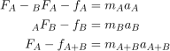
$\begin{aligned} F_A- {}_{B}F_A - f_A & = m_Aa_A \\ {}_{A}F_B - f_B & = m_Ba_B \\ F_A-f_{A+B} & = m_{A+B}a_{A+B} \\ \end{aligned}$

Conditioning the equations of motion:

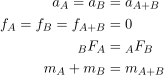
$\begin{aligned} a_A=a_B & =a_{A+B} \\ f_A=f_B=f_{A+B} & =0 \\ {}_{B}F_A & ={}_{A}F_{B} \\ m_A+m_B & =m_{A+B} \\ \end{aligned}$

and substituting numbers for symbols, write:

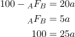
$\begin{aligned} 100 - {}_{A}F_{B} & = 20a \\ {}_{A}F_{B} & = 5a \\ 100 & =25a \\ \end{aligned}$

$\therefore$ The magnitude ${}_{A}F_{B}$ of the force that box $A$ exerts on box $B$ is $20\,\mathrm{N}$ .

May 27, 2022July 24, 2022

202205271015 Parametrization 001

equation $y=mx+c$ describes a straight line with slope $m$ and $y$ -intercept $c$ , as shown below:

With some scalar parameter $t$ parametrize the equation, in vector representation of units $\hat{\imath}$ and $\hat{\jmath}$ , by

$\mathbf{s}(t)=t\,\hat{\mathbf{i}} + (mt+c)\,\hat{\mathbf{j}}\quad\textrm{where } t\in (-\infty ,\infty)$

whereas for a quadratic equation $y=ax^2+bx+c$ which describes a parabolic curve, its parametric representation is

$\mathbf{s}(t)=t\,\hat{\mathbf{i}} + (at^2+bt+c)\,\hat{\mathbf{j}}\quad\textrm{where } t\in (-\infty ,\infty)$

and similarly for a circle of radius $r$ centered at the origin $O(0,0)$ , its locus is parametrized as

$\mathbf{s}(t)=r\cos t\,\hat{\mathbf{i}}+r\sin t\,\hat{\mathbf{j}}\quad\textrm{where } t\in [-2\pi ,2\pi ]$ .

(to be continued)

May 26, 2022July 24, 2022

202205261415 Arithmetic in Lisp

Given two operands $a$ and $b$ which are real numbers, define the operators,

$a+b$ , $a-b$ , $a\times b$ , $a\div b$ , $a^{b}$ , $\sqrt[b]{a}$ , $a\bmod b$ ,

with respect to arithmetic operations such as addition, subtraction, multiplication, division, exponentiation, rooting, and Modulo.

+------+------------+-----+-----+-------------------------+
|  ID  |  operator  |  a  |  b  |  instance for example   |
+------+------------+-----+-----+-------------------------+
|  1   |  +         |  2  |  3  |  a + b  = 2 + 3    = 5  |
|  2   |  -         |  5  |  2  |  a - b  = 5 - 2    = 3  |
|  3   |  ×         |  3  |  2  |  a * b  = 3 * 2    = 6  |
|  4   |  ÷         |  9  |  3  |  a / b  = 9 / 3    = 3  |
|  5   |  ^         |  3  |  2  |  a ^ b  = 3 ^ 2    = 9  |
|  6   |  √         |  3  |  8  |  a √ b  = 3 √ 8    = 2  |
|  7   |  mod       |  7  |  4  |  a mod b = 7 mod 4 = 3  |
+------+------ -----+-----+-----+-------------------------+

+------+------------+-----+-----+-------------------------+

| ID | operator | a | b | instance for example |

+------+------------+-----+-----+-------------------------+

| 1 | + | 2 | 3 | a + b = 2 + 3 = 5 |

| 2 | - | 5 | 2 | a - b = 5 - 2 = 3 |

| 3 | × | 3 | 2 | a * b = 3 * 2 = 6 |

| 4 | ÷ | 9 | 3 | a / b = 9 / 3 = 3 |

| 5 | ^ | 3 | 2 | a ^ b = 3 ^ 2 = 9 |

| 6 | √ | 3 | 8 | a √ b = 3 √ 8 = 2 |

| 7 | mod | 7 | 4 | a mod b = 7 mod 4 = 3 |

+------+------ -----+-----+-----+-------------------------+

Not so accustomed to these, Lisp cannot interpret or compile them until we have defined those seven primitive functions, better known as symbolic computations; as were newborn infants taught human intelligence by grownup adults between homo sapiens.

To Lisp, arithmetic operations are usually $\textrm{\scriptsize{NOT}}$ predefined. We have in our toolkit $\textrm{\scriptsize{ONLY}}$ three mathematical functors, i.e., list, iteration, and recursion.

The roots of quadratic equation are given by the formula:

$\displaystyle{x=\frac{-b\pm\sqrt{b^2-4ac}}{2a}}$

the expected outcome of which is calculated by parts, first the discriminant ‘delta’:

(define (delta a b c) (- (square b) (* 4 a c)))

1	(define (delta a b c) (- (square b) (* 4 a c)))

$\Delta = b^2-4ac$ ;

then the plus-minus ‘pm’:

(define (pm u v)
	(values (cons (+ u v) (- u v))))

1 2	(define (pm u v) (values (cons (+ u v) (- u v))))

$\pm (x)=(+x,-x)$ ;

and hence

(/ (pm (- b) (sqrt (delta a b c))) (* a 2))

1	(/ (pm (- b) (sqrt (delta a b c))) (* a 2))

will solve for real roots, ignoring the complex though.

$\therefore$ Predefining the seven primitive functions is in order for solving any computational problems by Lisp.

(to be continued)